Cascadia subduction zone creep
On April 29, 2014, I presented a talk for Data Rave, NYC at EBay. My collaborators on this project are Rob McCaffrey at Portland State University and Ken Creager at the University of Washington. This blog covers the talk, and the original slides can be found in my github repo. The paper for which the talk and this blog are based is found here. Like what you are reading? Check out my follow-up blog on slow slip and tremor!
A key question that geophysicists try to answer is “How much are tectonic plates “stuck” together?" The answer to this question has major implications on seismic hazard since it is thought that the more plates are stuck, the larger the earthquake will be. This blog will discuss how much the North American plate is stuck (or not stuck) to the Explorer, Juan de Fuca and Gorda plates within the Cascadia subduction zone, which resides in the Pacific Northwest corner of the United States.
First, I want to share with you the story of the blind men and the elephant because this story pretty much sums up my experience as a scientist, and my experience with this study (Figure 1). In the story of the blind men and the elephant, there were a group of blind men that decided to figure out what an elephant was really like, having never seen one before. So, they all approach the elephant from different angles and examine it. One blind man approaches a tusk and examining it declares, hey, an elephant is like a spear! But then another one came up to its wriggling trunk and decided it was more like a snake. In fact, each blind man made their own conclusion of what an elephant was really like having observed different parts of the elephant, but each of them only observed a small piece of the elephant. And so, these blind men all bickered about what an elephant really was like, and in reality they were all right because the elephant in fact has all of the properties the blind men said it had, but at the same time, they were all wrong because they weren't able to see the full picture.
Figure 1. Cartoon of the blind men and the elephant. G. Renee Guzlas, artist, source: http://www.nature.com/ki/journal/v62/n5/fig_tab/4493262f1.html
In this study I bring together interdisciplinary data sets, observed by myself and by other scientists in order to get a fuller picture of what is going on with the tectonic plates in the Cascadia Subduction zone. To my knowledge, this is the first study that brings together these datasets in a comprehensive way to better understand subduction zone mechanics.
Before diving into the research, I am going to quickly review some key concepts for this blog. Figure 2 is a map of the major tectonic plates that cover the earth. Each color represents a major plate. The plates rotate and translate with respect to each other all the time. The red arrows show how these plates are moving with respect to each other. They can move apart, which is what is observed in Iceland and mid-oceanic ridges. The plates can move laterally past each other, like the San Andreas fault, or, they can move toward each other. When an oceanic plate collides with a continental plate, the oceanic plate moves underneath ("subducts" beneath) the continental plate. These areas are known as subduction zones and they can produce some of the largest earthquakes in the world. These earthquakes can reach magnitude 9 or more on the Richter scale and can produce tsunamis. The 2011 Japan earthquake and the 2004 Sumatra Earthquake were examples of megathrust earthquakes (ie., large, magnitude ~9 earthquakes) that occurred in subduction zones.
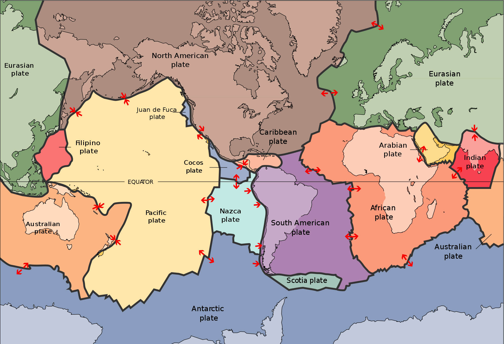
Figure 2. Major tectonic plates of the world. Image from http://www.sanandreasfault.org/Tectonics.html
This blog focuses on the Cascadia subduction zone, found in the Pacific Northwest of the United States. Figure 3 is a zoomed in view of the Cascadia subduction zone. The Explorer, Juan de Fuca and Gorda plates are currently being subducted beneath the North America plate. The last major earthquake occurred in 1700, and we know precisely when because of records of a tsunami in Japan (Atwater et al., 2005)! Scientists have estimated that this quake was approximately 1000km in length and the plates slipped about 20m (Satake et al 2003)! Yikes! The estimated moment magnitude for this quake was approximately 9.
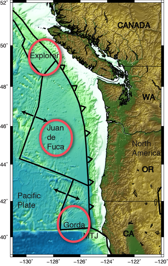
Figure 3. Close up map view of the Cascadia Subduction Zone. Topography data from ETOPO1 Topography Model. Figure made with GMT. Red circles outline oceanic plate names.
Let’s look a little deeper as to what is going on here. Figure 4 is a cross-section of the Cascadia subduction zone. You can see the Olympic Peninsula and Puget Sound. Below is an artist’s rendition of the Juan de Fuca oceanic plate subducting beneath the North America plate. The shallow, up-dip area is where the plates are thought to be stuck, or locked together. Further down-dip, the plates transition from fully locked, to fully creeping, where creeping is a measurement of how much the plates are slipping between large earthquakes. So, in the regions where the plates are stuck, lots of stress is building up, and is where megathrust earthquakes are thought to occur.
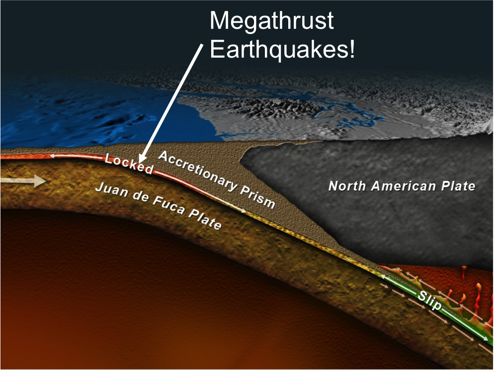
Figure 4. Profile cross-sectional view of the Cascadia Subduction Zone. Image from John Delaney.
So, what happens when the plates are stuck? The two plates are moving toward each other. In order to accommodate that motion, the two plates that are stuck together must begin to bend and deform. The continental crust begins to shorten and the ground near the coast begins to uplift.
When an earthquake happens, the two plates quickly slide past each other. The continental plate suddenly expands and subsides near the coast, and uplifts offshore. You can imagine the dire consequences of this – The uplifting crust shifts the entire water column up, possibly generating a massive wave which will eventually propagate to shore, but the shore line has also gone down, allowing the tsunami wave, once it hits, to reach further inland and be more destructive. As an example, Japan experience about 0.5-1 meter of subsidence during the 2011 quake (http://blogs.agu.org/mountainbeltway/2011/03/15/new-gps-vectors/) that also generated a tsunami that reached 33 ft high (http://en.wikipedia.org/wiki/2011_T%C5%8Dhoku_earthquake_and_tsunami). Yikes.
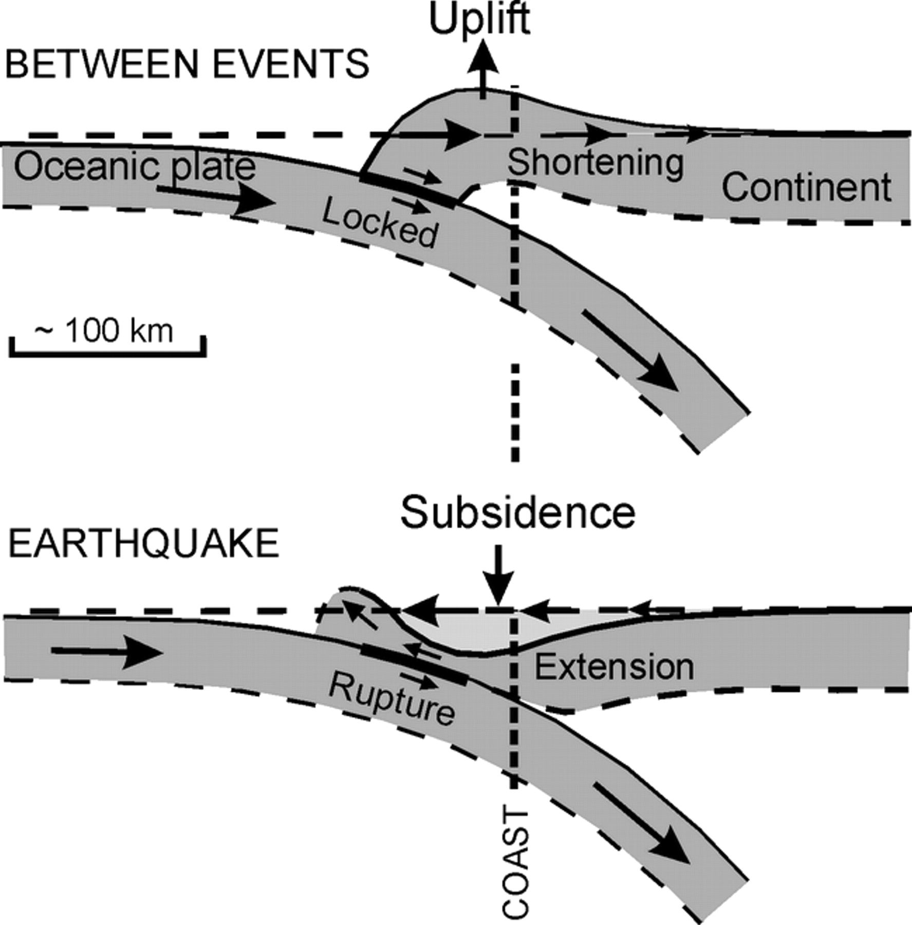
Figure 5. Cartoon of crustal deformation due to fault locking between earthquakes (top) and during an earthquake (bottom). Figure from Leonard et al., 2003.
The punch line of this study is that the amount of locking changes along the Cascadia Subduction zone--the plates are more stuck off the coast of Washington, southern Oregon and California, and less stuck in northern and central Oregon. This conclusion was reached by bringing together observations from a variety of cross-disciplinary studies, and like the blind men mentioned earlier, I attempt to piece together these data sets to make a simple, consistent story that explains all of them.
Let’s dive into the first data set – High precision Global Positioning Systems (GPS). A GPS satellite emits two wavelengths and some other information that help determine the distance of the satellite to a receiver on the ground (say your smart phone). It is important that two different wavelengths are emitted because it helps in calculating some distortions in the passing through the ionosphere. In the most simplistic view of how distance is calculated, one can take the time difference between the emission of the signal from the satellite and the detection of the signal at the ground reciever and multiply that differenced time by the speed of light. That will give the satellite line of site distance. To convert it to a 3 dimensional position, one would need the calculated range from at least 4 different satellites. There are currently 32 healthy GPS satellites in orbit, which means that any place on the earth, except maybe at the poles, can see at least 4 satellites at any given point in time.
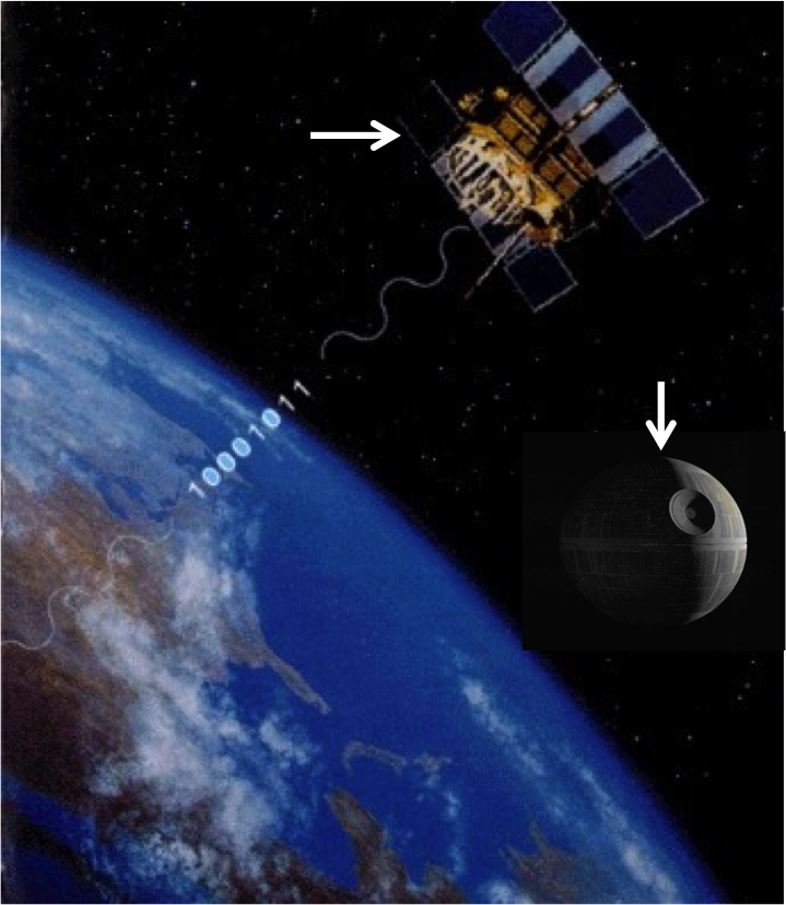
Figure 6. Horizontal arrow points to an image of a GPS satellite from http://www.geosoft-gps.de/english/gps_infos/info_2_e.html. Vertical arrow points to a picture of the Death Star. GPS satellites and the Death Star should not be confused.
Back here on earth, we have permanently installed GPS monuments. These guys are usually installed in bedrock, if possible, or some other sturdy structure. You may have seen some of these monuments, the top left corner of Figure 7 is an example of what one may look like. Below that is a Trimble 5700 GPS and a Zephyr Geodetic antenna – a little larger than your smart phone. The antenna is usually set up on top of a tripod that is centered over the monument. The right hand photo of Figure 7 shows the antenna on top of a tripod with a protective cover that helps keep snow off. The antenna detects the signals from the satellite, which is then sent to the connected receiver, that collects that information.
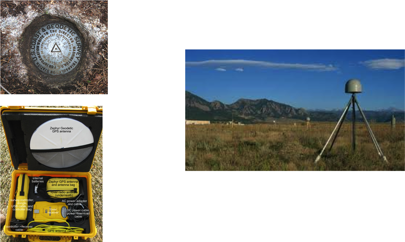
Figure 7. Upper left: photo of Geodetic monument from http://en.wikipedia.org/wiki/Survey_marker. Lower left: photo of a Trimble 5700 GPS and a Zephyr Geodetic antenna from http://facility.unavco.org/. Right: Picture of an operating GPS from https://earthdata.nasa.gov/featured-stories/featured-research/looking-mud.
Daily positions of the GPS can be estimated. Figure 8 is an example of a GPS position time series for its three components – North, East and Vertical. The blue dots mark the daily position estimate, and the vertical black lines the uncertainties. Interestingly at this particular site there was a small earthquake nearby which caused this jump in the position time series. But, you can imagine that, ignoring the earthquake we can calculate the rate at which this monument is moving by taking the slope of the time series for each component.
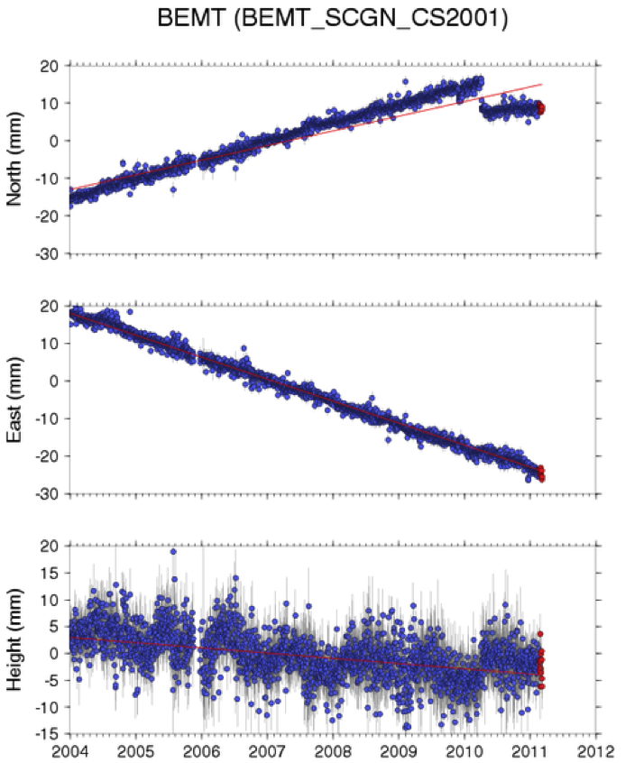
Figure 8. GPS position time series for site BEMT, taken from UNAVCO website.
Focusing on the horizontal velocities, we can estimate by eye that this site moved about 30 mm per 6 years, or 5 mm/yr. Similarly, we can estimate by eye that the north component moves at about 8 mm/yr. By taking the square root of the squares of these velocities we can calculate a magnitude and we can also calculate the direction it was moving by taking the arctangent of the two components. This gives you an idea of how a velocity can be calculated by eye. Calculating the time series velocities for this study is a little more rigorous, however, since other signals, such as earthquakes and seasonal effects convolute the velocity estimate. Using the least squares method, velocities in this study are calculated by fitting the time series to the linear linear equation:

- where
- p = position, po = initial position, v = velocity, t = time, H = Heaviside function (step function) for earthquakes or equipment changes, A = amplitude of offset, and U1-4 = constants for seasonal variations.
Another data set used was tide and leveling data from Burgette et al., 2009. Remember in between major earthquakes the region near the shoreline uplifts– which means it would look like sea level is lowering. This can be measured over time, and an estimate can be made on how much vertical movement happened over time.
Figure 9. Photo of a tide station. Photo from http://www.oco.noaa.gov/tideGauges.html.
Let’s look at the data! In Figure 10, the map on the left has horizontal GPS velocities that are estimated from daily position time series from 1997 to 2013. These velocities are referenced to stable North America, so you could imagine standing in Nebraska, looking longingly to the west coast, and watching the plates move as indicated by these arrows. The arrows here originate at the GPS monument, are sized according to their magnitude, and point in the direction of motion. Note the reference scale arrow in black is 5 mm/yr. Now let’s look at the vertical data set. For better illustration, I’ve color coded them so that warm colors represent more uplift. The key thing to notice about this data set is that there is more uplift in the north and in the south, and a reduced amount of uplift in central and northern Oregon.
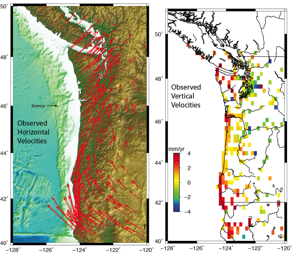
Figure 10. Maps of GPS horizontal velocities (left) and the combined GPS vertical velocities with tide and leveling uplift rates (right). Vertical rates colored according to their magnitude. Warm colors indicate uplift.
Geophysicists try to figure out how the world works by applying geophysical data to a mechanical model. What I mean is we think we know some basic concepts behind how the world works, so we build a mechanical model that will actually mimic what the earth is doing based on these concepts. One such model is called a block model. This type of model divides the corner of the earth you are working on into tectonic blocks that can move and rotate, strain and bend due to fault motions. We can use these models, along with the GPS data to estimate how much the plates are stuck together. The modeling program that I use is called TDEFNODE and it is a massive, wonderful beast of a code, written in Fortran! Yes, Fortran. It is based off of the models presented in McCaffrey et al., 2007. Figure 11 is a map of the Cascadia subduction zone with the block model geometry laid over top (solid black lines). The dots represent the interface between the subducting oceanic plate and the continental plate. It looks flat here, but really the fault interface is going down into the page.
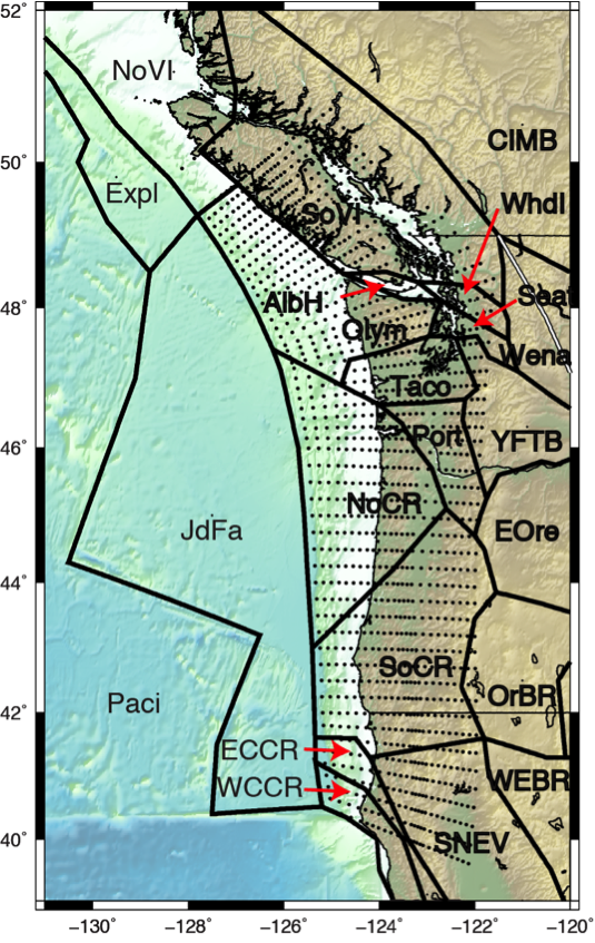
Figure 11. Geometry of three dimensional block model. Thick black lines mark block boundaries, dots the three dimensional subduction interface. Block names are labeled.
OK -- We have our data, and we have our model. Only we have a big problem – The locking, which is what we are trying to solve, is mostly offshore, where we don’t have any data to constrain the model! This means that the model is heavily reliant on the user assumptions. Hence, I've described the model in two ways -- The first I call the Gaussian model, which assumes that the locking is distributed along strike in a Gaussian way, where it is minimal at the trench, crescendos to a maximum, and then tapers off down-dip. The second way assumes that the fault is completely locked from the trench to some distance down-dip before it begins to taper off.
Figure 12 are maps of locking distributions for the Gaussian (a) and Gamma (b) models. The green lines mark the modeled block geometery, and the colors are the locking fraction – where red indicates that the plate are stuck together more, and the cooler colors mean that the plates are less stuck. The residuals for each model are nearly identical in both cases, even though at first glance these models seem very different. But let’s take a closer look here. Both models show much more intense locking offshore in Washington and in northern California and southern Oregon. And the other distinguishing feature is that there is a wide transition zone between about 43 and 46 degrees north in central and northern Oregon. So, for these models, locking must be reduced in order to fit the reduced GPS, tide and leveling uplift rates in this region.
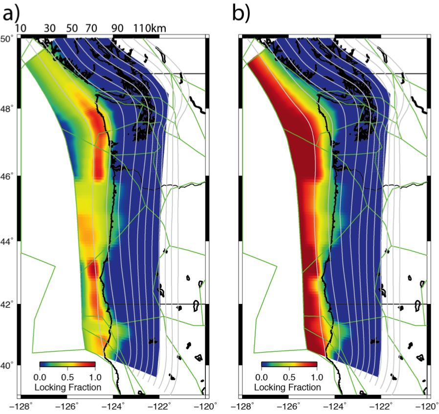
Figure 12. Locking distributions for the Gaussian (a) and Gamma (b) locking distribution models. Green lines mark block model boundaries, warm colors indicate regions that are more locked.
Up until now we have been talking about what happens in between major earthquakes. Let’s change gears a bit and think about what happens during an earthquake. Remember that during an earthquake, the continental crust uplifts offshore, potentially displacing the water column and producing a tsunami. Near the coast the ground subsides, allowing tsunami waters to inundate the shore line much further than in between earthquakes, bringing with it sediment and debris that would eventually settle out of the water column and form a geologic layer. These tsunami deposits can be seen in the geologic record. From these geologic layers, paleoseismologists can deduce how much subsidence occurred. Diatoms and other organic matter can help date when these layers were formed.
Leonard et al., 2010 compiled subsidence records from a plethora of studies that include earthquakes from the past 6500 years in Cascadia. Figure 13 shows a subset of subsidence data from some of these Cascadia earthquakes. The figure displays subsidence as a function of latitude, ranging from 50 degrees latitude (Canada) to 40 degrees latitude (northern California). What Leonard et al., 2010 observed is that for multiple past earthquakes, subsidence was reduced between 43.5 and 46 degrees north latitude. In their study, they state that reduced subsidence in central Cascadia is a persistent feature of Cascadia subduction earthquakes.

Figure 13. Subsidence records compiled in Leonard et al., 2010. Reduced subsidence is observed between ~43.5 and 46 degrees North.
Hmmph...
So let’s recap what we have so far – in the same region, at about 43-46 degrees north, we have both reduced inter-earthquake uplift as well as reduced subsidence due to earthquakes!
Now we come to my elephant -- that is, my interpretation of these observations. One way we can explain these observations is by fault creep in central Cascadia. In the locked scenario, the two plates are pushing together, creating uplift, which we see in Washington and California. This builds up a lot of stress which is later released in a big earthquake (Figure 14). In the case where the plates may be partially creeping the two plates are actually sliding past each other in between major earthquakes and stress doesn’t accumulate to the same extent – this means that we are less likely to see as much uplift in between earthquakes, and when an earthquake does happen the slip is expected to be less since much of it was already accommodated between earthquakes (Figure 14).
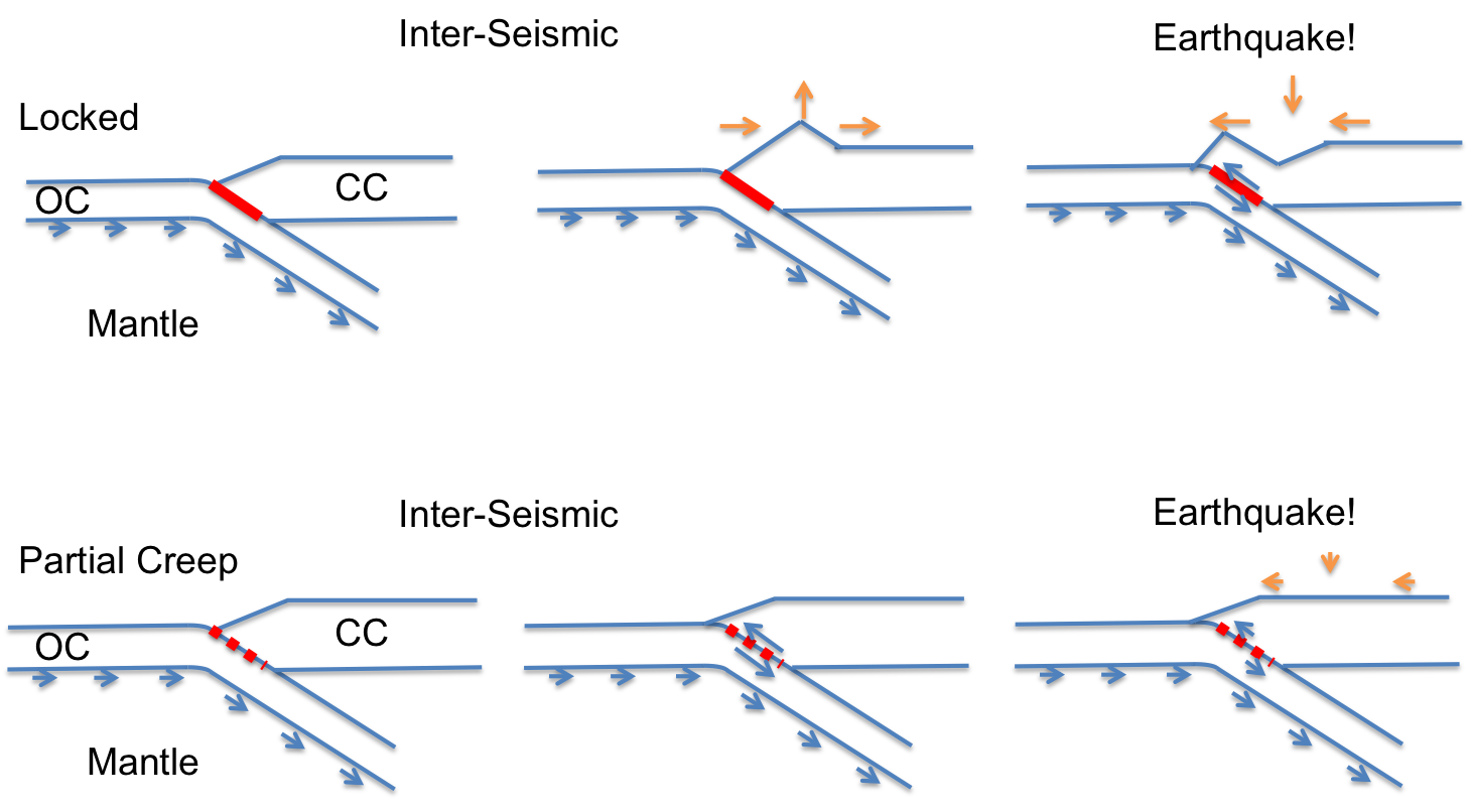
Figure 14. Subduction zone locking and creep scenarios. The top row shows the expected deformation for a locked subduction zone -- the continental crust uplifts near the coast in between earthquakes, and experience lots of subsidence during an earthquake. Alternatively (bottom row), if the subduction zone is creeping then the two plates release stress between earthquakes so that when an earthquake happens less slip is expected.
So, now we have our theory, based on interdisciplinary research using GPS, tide gauge, leveling and paleoseismic datasets. The theory, however doesn't explain why the plates are creeping in central Cascadia. Burgette et al., 2009 present a model similar to the Gamma model above, but they enforce a narrow locking transition width. In order to fit the reduced uplift rates in central Cascadia, their model shifted the locked region offshore. They note that the locking pattern in their model correlates well with the location of a dense, Eocene age (~50 Ma) accreted basalt known as the Siletzia terrane, and suggest it may influence the locking. The Siletzia itself is pretty rigid -- it has few earthquakes within its body (Parsons et al., 2005). Some studies suggest that it may also be less permeable (Calkins et al., 2011). Seismic surveys indicate that the Siletzia terrane is thickest in coastal Cascadia in central Oregon, where it extends as much as ~35km offshore. In Washington, the Siletzia terrane is not present in large quantities in the Olympics, but is observed further east in the Puget Sound region (Parsons et al., 2005).
Because the Siletzia terrane is dense, it can be mapped in gravity surveys. Blakely et al., 2005 present gravity data sets that map out the extent of the Siletzia terrane. We use the 10 mgal contour line of this data set to map out the thickest accretions of the Siletzia terrance (Figure 15). The gravity anomaly outlined shows the largest block extends from about 44 to 46 degreen north latitude, and extends through our region with reduced interseismic uplift and reduced coseismic subsidence. The outline is mapped on top of the Gaussian locking distribution model in Figure 15, but please note that their is no preference between model solutions.
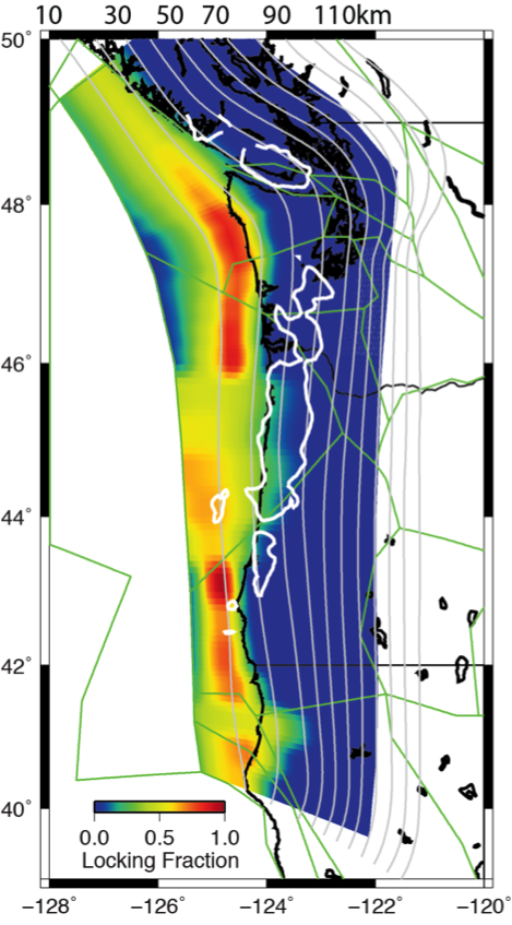
Figure 15. Gaussian locking distibution model plotted with 10 mgal contour line (white line) from Blakely et al., 2005.
This study builds off of a conceptual model from Reyners and Eberhart-Phillips, 2009. In their study of locking distributions in the Hikurangi Subduction Zone (HSZ) under the North Island of New Zealand, they note that the less permeable Rakaia terrane, seems to also be influencing the locking. They suggest that the impermeable Rakaia terrane prevents water generated from the basalt-eclogite transition from percolating up into the overriding crust. Instead, pore fluid pressures increase at or near the plate interface and influences the locking. Intriguingly, their study suggests that the Rakaia terrane is more locked than its surroundings. We suggest a similar conceptual model for Cascadia, where the Siletzia terrane, if impermeable, increases pore fluid pressures by not allowing water to percolate into the overriding crust. We suggest, however, that the high pore fluid pressures at or near the plate interface encourages creep, since these conditions are thought to favor stable sliding (Segall and Rice, 1995; Hillers and Miller, 2006.
So, here is the recap of this work:
- We observe reduced interseismic uplift rates in central Cascadia determined with GPS, tide and leveling data sets. Models of plate interface locking indicate that locking has to be reduced with a wide transition zone (this study) or move offshore in order to fit these data.
- Paleoseismologists observe reduced coseismic subsidence from past great earthquakes in central Cascadia.
- The above observations can be explained by creep in central Cascadia.
For a deeper discussion of the observations and hypotheses presented in this blog, please read Schmalzle et al., 2014.
Thanks for reading!
Like what you read? Check out my follow-up blog on periodic slow slip and tremor!
Acknowledgments: This work was funded by the National Science Foundation (NSF) Postdoctoral Fellowship Program, award 0847985 (Schmalzle), NSF award EAR-1062251 (McCaffrey), and USGS National Earthquake Hazards Reduction Program, Award G12AP20033 (Schmalzle and Creager). Some of the figures I made myself using General Mapping Tools (GMT), but some figures I took from random places on the web. For any of those images I say where the figure was taken. Many thanks to Reed Burgette and an anonymous reviewer for their thoughtful comments and suggestions that greatly improved this research. Thanks to Rick Blakeley for providing gravity data. Craig H. Faunce, Bruce Nelson, Steve Malone, Justin Sweet, David Schmidt, Aaron Wech, Tom Pratt, Brian Atwater, Sarah Minson, Lorraine Wolf, and Aimee Schmalzle provided useful comments and insight. Thanks to PBO and PANGA for providing access to GPS data products. Special thanks to David Branner, Ruby Childs and Nick Collins for organizing Data Rave and inviting me to give a talk.
Comments
comments powered by Disqusblogroll
social