Generic Mapping Tools

Update, Feb. 7, 2015: A comment made by Joseph below alerted me that I had been referring to GMT as General Mapping Tools, which was incorrect! The correct name is Generic Mapping Tools and has since been updated. Many thanks to Joseph for pointing this out, and my apologies for my gaffe! BTW -- I love the commentary -- it provides great feedback for improving my blog. Please don't be shy!

Original (Revised) Text:

Before my time here at Hacker School I put together a short, hands on course on how to use Generic Mapping Tools (GMT). GMT is a very powerful mapping and data visualization package. This class was based around using GMT 4. GMT 5 has slightly different syntax and functionality and will not work with the scripts presented here. I intend to update the scripts to GMT 5 in the near future.

The class was taught at the University of Washington Earth in the Department of Earth and Space Science, so it has an earth science theme -- earthquakes! Here, students learn how to make a map with layers that include mapping topography and earthquake locations. A subset of data is extracted from a profile line (red line in map below) so that earthquake depths can be plotted as a function of distance. The end goal of the class is to produce the following map and transect:

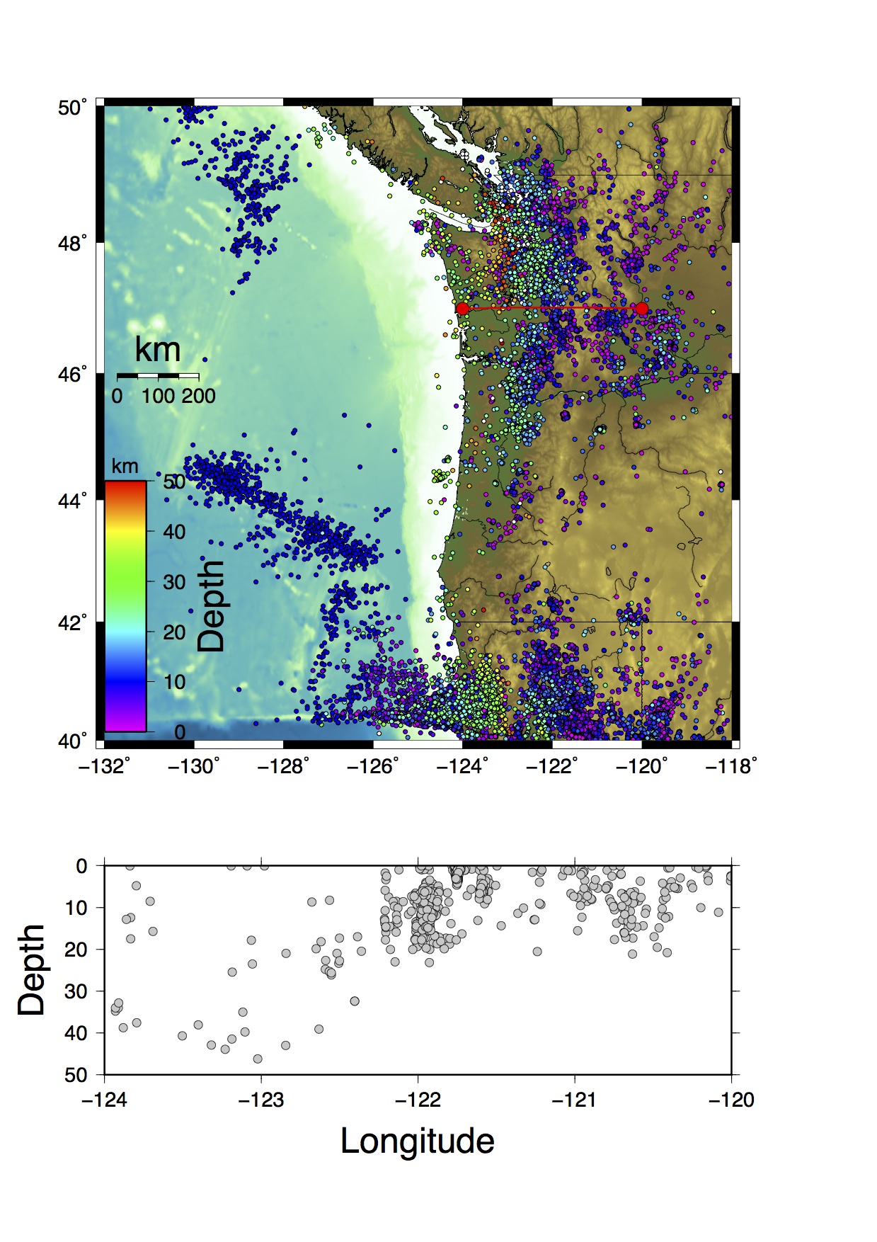
Figure 1. Map of the Cascadia subduction zone in northwestern United states overlain with ETOPO1 topography model (relief map), and earthquake locations from the ANSS catalog (circles) colored according to earthquake depth. Red line marks profile line from which data are extracted and plotted the depth vs. longitude graph below the map.

All files are contained in my Github repo except for the ETOPO1 topography model dataset. Unfortunately, this is a gigantic file that I could not push to the github repo without errors. The grd file can be downloaded on the original website, however, at http://www.ngdc.noaa.gov/mgg/global/relief/ETOPO1/data/bedrock/grid_registered/netcdf/ETOPO1_Bed_g_gmt4.grd.gz.

The file that made the above figure (cascadia_seis.com) is also in the repo, but I am also including a very verbose version below that goes through and explains each step, including some basics of bash scripting:

#!/bin/bash
# This file is for the first class on data visualization with GMT
# Written by Gina Schmalzle
# This code is a bash shell script (http://en.wikipedia.org/wiki/Bash_(Unix_shell)) that calls GMT files.
# awk is used to manipulate data files (http://en.wikipedia.org/wiki/AWK).

# A unix shell is a "command line interpreter" that allows definition of variables,
# and execution of commands that could be done via the command line.  A nice shell script
# will make it easier to change variables, and easier to implement several lines of code.
# Shell scripts are commonly used with GMT programs.

# Most if not all of the commands in this document have associated 'man' (manual) pages.  To access them type:

# man whatever_your_command_is

# If you cannot access your man pages through your command prompt, an alternative would be to type man command in
# google.

# To make this file executable, you will have to change the mode of the file (ie, read, write and/or execute)
# In your directory you will need to type:

# chmod u+x ./cascadia_seis.com

# The '#' marks to the left indicates a comment.  Anything written after them is not read when the file is executed.

# This file will create a map of Cascadia that includes a grid of topography data from ETOPO1 (ETOPO1_Bed_g_gmt4.grd) and
# seismicity data.  These data will be applied in "layers", very similar to how GIS packages have layers.  The layers may be
# turned off or on by commenting/uncommenting lines.

# The grd file is already in gmt format.  Generating and using grids is another class in itself, but here I will introduce
# you to using GMT formated grid files.

# Also included on the map are earthquakes locations color coded by depth from the ANSS catalog for 2000 to 2012 (anss_eq_2000_2012.dat)


#MAKE A MAP!

# Define the names of the input and output files
out=cascadia_seis.ps                           # This will be the name of your map generated by this file
seis_data=anss_eq_2000_2012.dat                        # ANSS earthquake catalog
topo=./ETOPO1_Bed_g_gmt4.grd                   # ETOPO1 topography grid

# Define map characteristics
# Define your area
north=50
south=40
east=-118
west=-132

# Define your map boundary annotation
# Here we define tick marks every 2 degrees and we print the degree on the West and South sides of the plot
# and keep the ticks (but don't label) on the east and north sides
tick='-B2/2WSen'

# Define Map Projection
# Here we define a Mercator Projection of size = 15
proj='-JM15'

#Start with GMT commands with embedded definitions....
# Help with any of these commands can be obtained by looking at the 'man' files.  Simply type at the command line: man gmt_command
# If the man files are not properly installed you can also type in man gmt_command (e.g., man psbasemap) in google and it will come up.

#This line sets up the 'basemap' meaning  here you will define the region, boundary annotations and projections.
#You can accomplish this also with other commands (including psxy, pscoast, etc...), but it is good many times to start with psbasemap.

psbasemap -R$west/$east/$south/$north $proj $tick -P -Y12 -K > $out

# This is your first line of GMT Code!!! Whoo-hoo!  In long hand this line would look like this:
#
# psbasemap -R-132/-118/40/50 -JM15 -P -Y12 -K > cascadia_seis.ps

# What the options mean:
# psbasemap = plots postscript basemaps
# -R -- defines the area of your map (note that we defined north, south, east and west above and they are inserted into the -R option.
# The Projection (-JM) and tick marks (-B) were defined above.
# Note that when you call a defined variable, you must include a '$' before the variable name
# -P Sets the figure to "Portrait" mode.  No -P is landscape.
# -Y Orients the figure vertically (-X orients it horizontally).
# -K means that there will be more 'stuff' appended to the postscript file.
# '>' means that the command output, which would normally print to screen will be directed into your new file (cascadia_seis.ps, shown here as $out)
# In addition it means that it believes cascadia_seis.ps is a new file.  If it is not, it will erase all existing info in the file and re-write it with
# the new information.


#plot grid
# We would like the topography to be the map background, so it needs to be the first layer.  Hence, we get started with a hard part...

# Helpful hint...
#
# use grdinfo  your_grd_file.grd
# to find info about your grid file, such as the min and max values
#
# You will need to make some color palettes.  These are files that tell what colors certain properties are displayed.
# For example, your ETOPO grid has a latitude, longitude and a elevation, and you want to color code the topography
# by elevation.  The following lines will tell you how to do that...

# First, Make a color palatte
# Typing:  makecpt
# at the command line will give you information on pre-existing color schemes
# This will make a color pallete of typical, pre-defined topography colors:

makecpt -Crelief -T-8000/8000/500 -Z > topo.cpt

#makecpt = makes GMT color palette tables
#-C tells GMT what pre-defined color palette to use
#-T defines the range and increment
#-Z states that the colors will change continuously (rather than discretely)
#topo.cpt is a new file containing your color pallete information that will be used later.


#This next line is not necessary, but may be used to make the image appear sharper.
#grdgradient helps to illuminate ridges in the topography from a specified angle.
#grdgradient $topo -A135 -Ne0.8 -Gshadow.grd

#grdgradient=Makes illumination shadow
#-A is the angle from which the light is shown
#-N normalizes the shadow according to equations stated in man grdgradient
#-G lists the name of your output grid


# Overlay the grid onto your map
# Here you are adding the grid as a layer to your postscript file

# This command includes a shadow grid file:
# grdimage $topo -R -J -O -K -Ctopo.cpt -Ishadow.grd  >> $out

# This command omits the shadow file:
grdimage $topo -R -J -O -K -Ctopo.cpt   >> $out

#grdimage = creates an image from a 2D netcdf grid file
#-R = Sets the region.  Notice here I don't have to state the min and max values again.
#-J = Sets the projection.  Again the type and size don't have to be restated.
#-O = Overlay. The output for this line is being appended to a previous postscript code
# i.e., you are adding another layer
#-K = You will be appending another layer
#-C = You will be using the color pallete topo.cpt

# Now, back to the easy stuff..
# Add coastlines

pscoast -R -J -O -K -W2 -Df -Na -Ia -Lf-130.8/46/10/200+lkm >> $out

#pscoast = adds coastlines
#-W = Sets the line width and color.  Default color = black = 0 and does not have to be explicitly stated.
#-Df = What is the resolution of the coasline dataset?  f = fine
#-Na = Draws politcal boundaries, a = draw all the boundaries, see man pscoast for more options
#-Ia = Draw Rivers, a = draw all rivers, see man pscoast for more options
#-Lf = Draw a fancy map scale, f = fancy, centered on -130.8, 46 degrees. +200 = length, +lkm = kilometers


# Add seismic locations and color code them by depth
# Make color palette
# Ahh, another color pallete...
# This time, let's make it rainbow colored and call is seis.cpt

makecpt -Crainbow -T0/50/10 -Z > seis.cpt

# Columns 4, 3 and 5 of the data file are the longitude, latitude and depth, respectively.  This is the order
# your data need to be in for psxy (see man file)

awk '{print($4,$3,$5)}' $seis_data | psxy -R -J -O -K  -W.1 -Sc.1 -Cseis.cpt -H15 >> $out

# psxy = Plot 2D lines, polygons and symbols on a map.  Fun fact -- psxyz plots in 3D.
# -W.1 = Draws the black outline of the circles.
# -Sc.1 = Defines the shape and size; c = circle, size = 0.1
# -H = Header.  The first 15 lines of the file contain header information and will not be read.
# -C = defines the color palette to be used for the depth.  We could also make all the circles one color.
# In this case, remove the -C option and use -G instead.  -G defines the color of the circle in either white-black
# or red/green/blue format.  Example colors:  -G0 (black); -G255 (White); -G255/0/0 (Red)
# GMT has made this a little easier.  You could also say -Gblack or -Gred, but there are a limited amount of colors
# you could do that with.


# Add a scale
psscale -D0/3.2/6/1 -B10:Depth:/:km: -Cseis.cpt -O -K >> $out

# pscale = Adds a scale to go with your color palette
# -D = set the position of the scale
# -B = set and annotate the scale tick marks and lables.
# -C = specify your color palette



# Now, let's take a subset of seismic data and project them onto a line....
#First, let's view the transect line

#Plot transect line
psxy center.dat -R -J -O -K -W1 -Sc.3 -G255/0/0 >> $out
psxy center.dat -R -J -O -K -W5/255/0/0 >> $out

# You should know the options by now ;-)

#This ends the map making part of this exercize, now we move onto making a scatter plot from the seismic data.



# PROJECT DATA
# Here we use the GMT code project to take all the data within a certain region and project them onto a line

awk '{print($4,$3,$5)}' $seis_data | project -C-124/47 -A90 -W-.2/.2 -L0/4 -H15 > projection.dat

# project = projects data onto a transect
# Note that the options are different for this command
# -C = defines the center of your transect
# -A = azimuth of transect (CW from N)
# -W = Width of the transect in degrees
# -L = length of transect in degrees
# -H = Header declaration
# projection.dat = new file with the original data and the projected locations




# MAKE SCATTER PLOT
#We want the scatter plot to be on the same page as the map, but just below it, so we need to redefine our
#region, projection and tick marks...

east=-120
west=-124
dmin=0
dmax=50

proj=-JX15/-5
tick=-B1:Longitude:/10:Depth:WSen


awk '{print($6,$3)}' projection.dat | psxy -R$west/$east/$dmin/$dmax $proj $tick -W1 -Sc.2 -G200 -O -K -Y-8 -P >> $out


# Columns 6 and 3 are the projected longitude and the Depth, repectively
# -Y = Shift the new plot down 8 units.  You can designate if you want to shift in centimeters (c), inches (i),
# meters (m), or pixels (p).  Otherwise it shifts by whatever is in your gmtdefaults.

# Last, but not least, image your map!
# Common postscript viewers:  gs, gv, ggv, open, gimp
# What, you don't like postscript files?  That's ok, uncomment this line:
# ps2pdf $out

open $out