Cascadia subduction zone creep

This blog is a continuation of the original 'Why the Cascadia Subduction Zone is Creepy' blog posted a few weeks ago, and many of the terms used in this post are defined there. My collaborators on this project are Rob McCaffrey at Portland State University and Ken Creager at the University of Washington. The paper this blog is based on is found here.

The Cascadia subduction zone is not just creepy, but it is creepy on many different levels (Figure 1).

Figure 1. I had to include this figure. So funny, I laughed for hours, and I'm not even a fan of pet photos.

No, I don't mean that kind of creepy. What I mean is that the tectonic plates that make up the Cascadia subduction zone between major earthquakes are in some places stuck together, but in others are partially slipping (aka, creeping). My previous blog talks about regions on the subduction fault that are stuck (or 'locked'), and regions undergoing persistent fault creep between major earthquakes, where persistent fault creep means just that -- between earthquakes the plates are constantly, slowly slipping. However, there is yet another slip phenomenon that periodically occurs between major earthquakes called slow slip, and is the topic of this blog.

Figure 2 is a cross section of the Cascadia subduction zone that shows the Juan de Fuca plate subducting beneath the North America plate. On the up-dip portion of the fault, the plates are stuck in between large earthquakes. This region is expected to be where the next megathrust earthquake (magnitude ~9) will occur. Much further down-dip, the plates slide freely past each other. Between these two regions, however, it was fairly recently discovered using continuously recording GPS that the two plates periodically slip over a period of weeks to months (Dragert et al., 2001), and in doing so accumulate enough slip to be equivalent to moment magnitude 6-7 earthquakes! Interestingly, you can't physically feel these periodic slow slip events (or SSEs) because they happen so slowly compared to an earthquake, which can last for a few seconds to minutes. Major slow slip events happen every 10 to 24 months, depending where you are observing along the Cascadia subduction zone. We will talk about how often these events occur a little later in the blog.

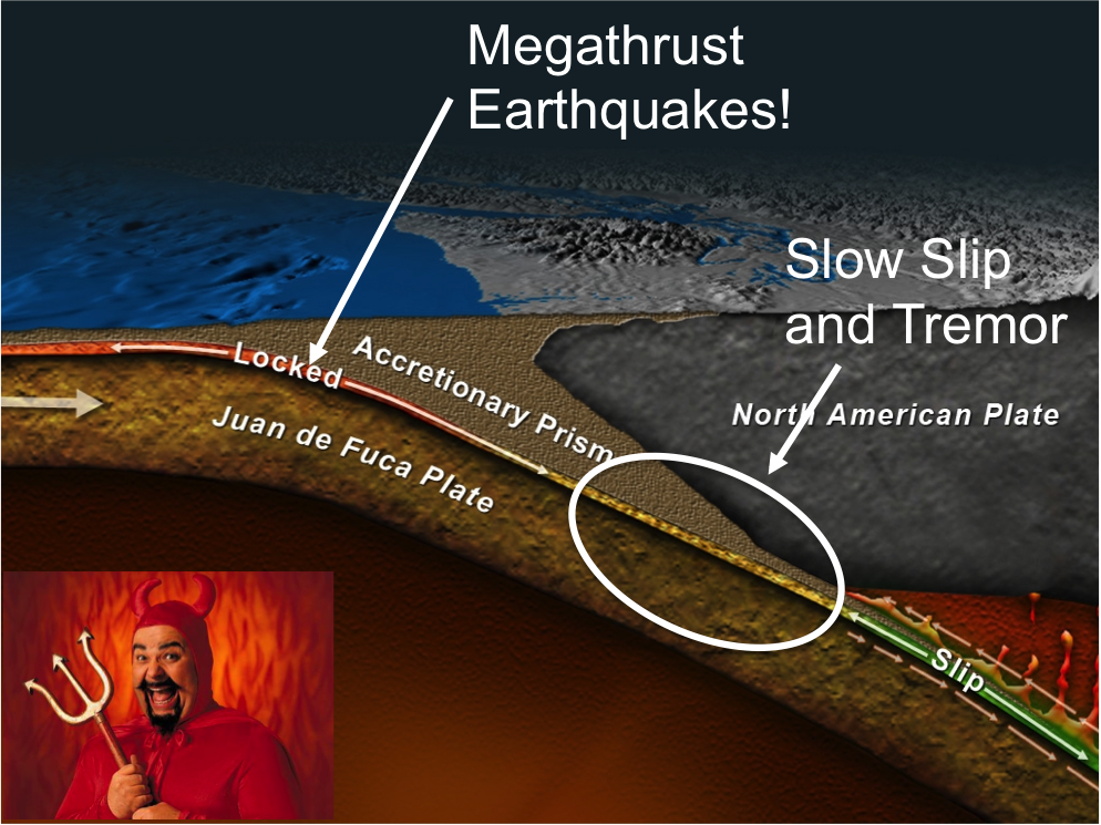
Figure 2. Cross-sectional view of the Cascadia Subduction Zone. Image from John Delaney. White oval indicates region that experiences slow slip and non-volcanic tremor. The little devil guy, that is courtesy of too much coffee. Thanks to Aaron Wech for giving me the idea (BTW -- that is not Aaron Wech in the photo, though maybe it should be...).

Not too much time after the discovery of SSEs, periodic bursts of noise were observed at nearly the same time among multiple local seismometers (Figure 3).

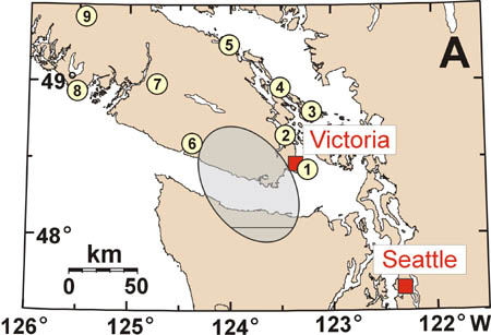
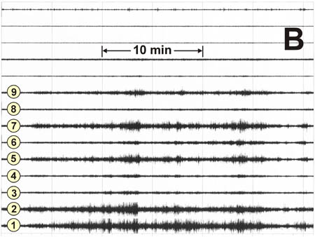
Figure 3. Figures modified from the Natural Resources Canada webpage. (A) Map of seismometer network. (B) Example seismic records for corresponding seismometers located in (A).

Soon scientists realized what they were seeing wasn't noise at all -- it was actually a seismic signal generated from these periodic SSEs that became known as non-volcanic tremor, sometimes referred to simply as tremor. Figure 4 demonstrates how well in time the non-volcanic tremor correlates with GPS detection of periodic slow slip. The blue dots in Figure 4 are the east component positions of a GPS site on Vancouver, WA. The time series produces a saw-tooth pattern. Each drop indicates that the motion of the station temporarily reverses (indicating an SSE). Non-volcanic tremor activity is also plotted on Figure 4 and shows that the non-volcanic tremor peaks during these GPS detected SSEs.

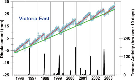
Figure 4. Modified from the Natural Resources Canada webpage. Blue circles are daily east position time series of a GPS site near Victoria. The green line is the long term eastward motion of the site (with respect to North America), and the red saw-tooth line shows the motion of the site between events is faster than the long-term motion. The bottom black line shows the number of hours of tremor activity observed on southern Vancouver Island.

The combination of periodic slow slip and non-volcanic tremor together was coined by the Canadian Geologic Survey as 'Episodic Tremor and Slip (ETS)' (Rogers and Dragert, 2003). Intriguingly, non-volcanic tremor and SSEs are not observed together or at all for all subduction zones, but that is a topic for another blog.

Subsequent studies have shown that in Cascadia ETS recurrence varies along strike of the subduction zone. Figure 5, (from Brudzinski and Allen, 2007) color codes select continuously recording GPS (squares) and broadband seismometers (triangles) by how often they detect periodic slow slip and tremor, respectively. Warmer colors indicate the site detected them more often. What Brudzinski and Allen, 2007 found is that ETS recurrence seems to be segmented along the margin, with ETS events happening every ~10 months in northern CA, ~24 months in central to northern Oregon, and about every 14 months in Washington (Figure 5).

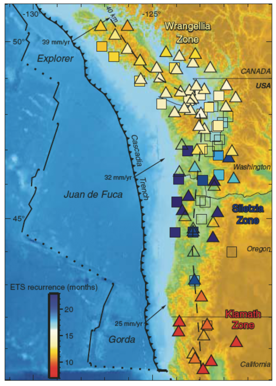
Figure 5. Map of the Cascadia subduction zone modified from Brudzinski and Allen, 2007. Squares and triangles represent locations of high precision GPS and broadband seismometers, respectively, and are colored by how often slip and tremor are detected.

So the recurrence of these events are not the same along the margin, but does that mean that the amount of tremor and slip along the margin also differ? First, let's look at the tremor. The Pacific Northwest Seismic Network, operated out of the University of Washington, keeps a continuously updating catalog of tremor along the entire margin. For some interactive tremor fun, you might want to check out their tremor mapping tool. Figure 6 is a tremor density map -- in other words, it takes how many tremors were detected over a specified region (the squares on the map), applies that number to a color scale that is then used to color the region. Dark blue colors indicate regions where the tremor counts are higher. Correlating well with the how often tremor and SSEs are detected, tremor counts for the time period of August 2009-August 2013 (2009.6-2013.6) are elevated where the recurrence time is shorter and lower where the tremor and SSEs are detected less (Figures 5 and 6).

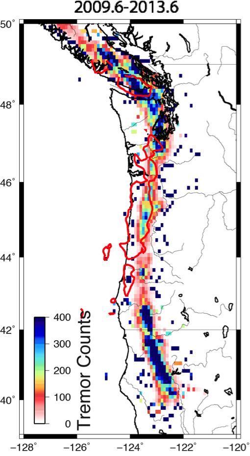
Figure 6. Non-volcanic tremor density map of the Casacadia subduction zone. Tremors from August 2009-August 2013 are used. Tremor counts larger than 400 are colored blue. Tremor locations from the Pacific Northwest Seismic Network tremor catalog. Solid red line marks the 10 mgal gravity anomaly from Blakely et al., 2005.

So what about periodic SSEs? The total amount of slip on a fault due to periodic SSEs over time is a little more difficult to estimate because our observations are on the surface of the earth, but we really want to know what is going on down on the fault. In order to figure that out, we will need to build a mechanical model, but we will get to that part in a minute. For now, let's take a look at the data. In Figure 4 the east component GPS time series of a site in Vancouver, Canada is shown. The GPS east position time series in this figure has a slope (notice that the time series position starts at about 1996 at -5 mm, and ends in 2004 at about 28 mm. The slope (calculated by eye) is then (28mm- -5mm)/(2004-1996) = 33mm/8yrs = 4.125 mm/yr). This slope marks the long term velocity of the time series, which is illustrated in Figure 4 as a green line. Notice that in between slow slip events the slope is larger (red line), and indicates the inter-SSE velocity, which in Cascadia seems to be pretty consistent between SSEs. To better visualize the GPS offsets from SSEs along the Cascadia subduction zone, the inter-SSE velocity is simply subtracted from the time series. Figure 7 displays the time series from select sites from Canada down to northern California. Note that the SSEs (marked by jumps in the time series) are well defined and fairly frequent in the north, reduce in amplitude and recurrence as we enter Oregon, then pick up again as we move into southern Oregon and northern California. South of about 40 degrees latitude SSEs are not detected with GPS.

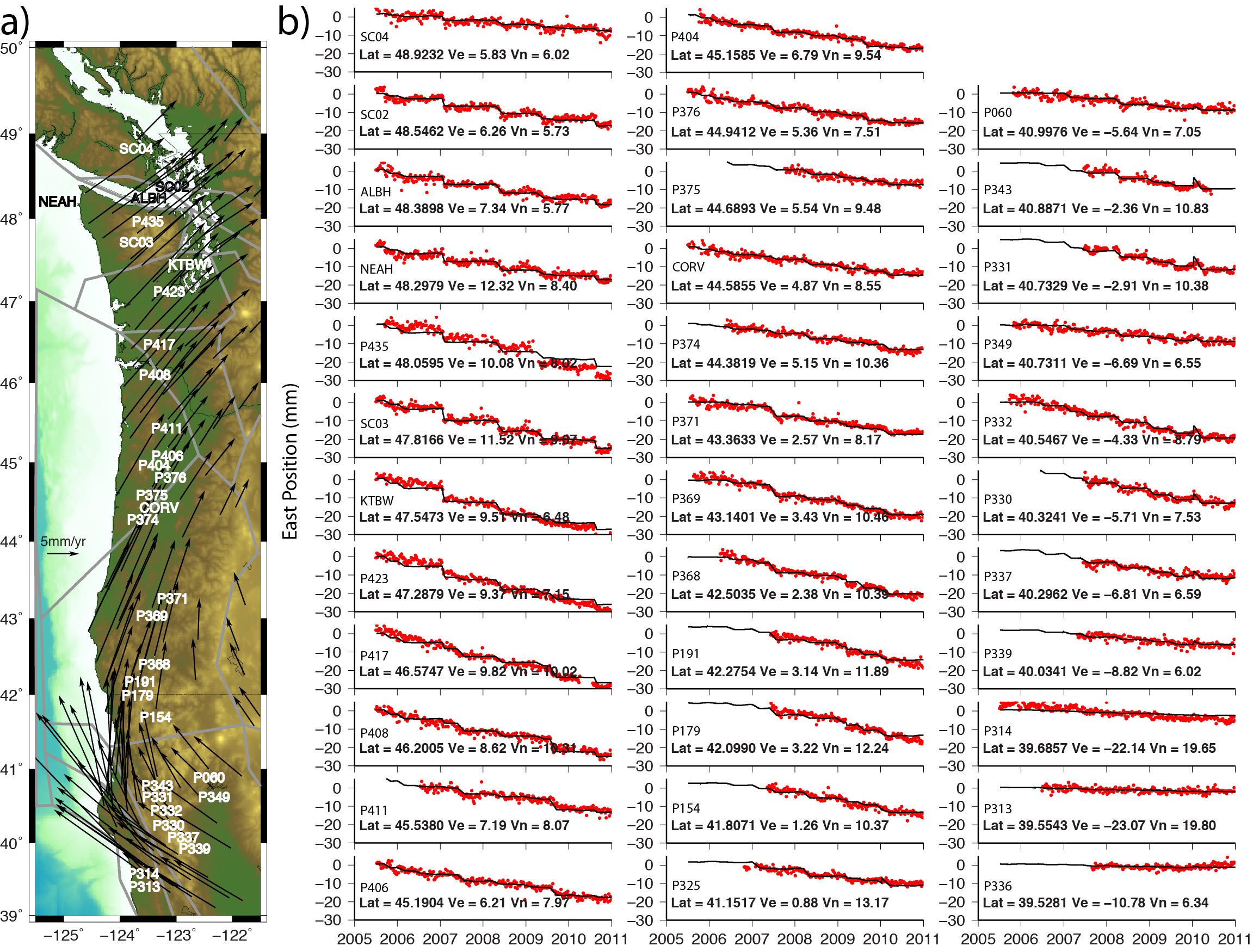
Figure 7. Map of inter-SSE GPS velocities (black arrows) with select GPS monuments labeled (a). East component of detrended GPS position time series (red dots) with model fit (black line) for sites labeled on the map (b). The site name, latitude of the site (Lat), and the east and north velocity components (Ve and Vn, respectively) are given. Figure from Schmalzle et al., 2014.

Now, let's get into how we figure out what is going on at the fault during the SSEs. As mentioned previously, the GPS position time series are observations on the surface of the earth, but we would like to know how much periodic slow slip is occurring on the fault. Similar to my previous blog, we use a mechanical model. To briefly review, a mechanical model mathematically mimics the behavior of the earth and the math behind these models are based on what we think the earth is doing. In the previous blog, we used a mechanical block model to explore how much the tectonic plates are stuck in between earthquakes, but in this blog we are interested in seeing how much and where the plates are slipping during SSEs. We again use the block modeling software TDEFNODE, which breaks up the region of interest into tectonic blocks (Figure 8). Instead of using the long-term pre-estimated GPS velocities with the model we use GPS time-series directly. What I want you to take away here is that the model mimics how much the tectonic plates are stuck between the SSEs, and how much they slip during the SSEs. It estimates slip for 16 SSEs that occur between 2005.5 and 2011 throughout the Cascadia subduction zone. The goal here is to add up all the SSE slip from that time period and see how it changes as we go from north to south. For details on the modeling, please refer to Schmalzle et al., 2014.

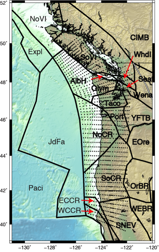
Figure 8. Geometry of the three dimensional block model. Thick black lines mark block boundaries, dots the three dimensional subduction interface. Block names are labeled.Figure modified from Schmalzle et al., 2014.

Now let's look at the results! The black lines in Figure 7b GPS position time series are modeled east positions over time for points that colocate with the observed GPS monuments. Figure 9 are examples of model estimated fault slip patterns for two SSEs in 2007, plotted next to tremor detected during the same time period.

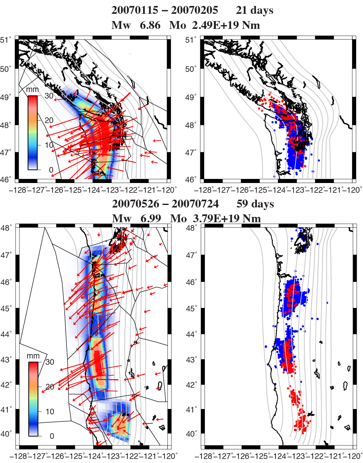
Figure 9. Slip distributions for two SSEs in 2007 estimated using the block model. The left-hand images show slip patterns (colors) overlain with estimated GPS displacement vectors for that event (red arrows). The images to the right show non-volcanic tremor locations that occurred in the same time period as the SSEs. Blue dots are tremor from the Pacific Northwest Seismic Network, and red dots are tremors from the Miami University catalog, courtesy of M. Brudzinski. Figure modified from the Supplementary material of Schmalzle et al., 2014.

As expected, Figure 9 shows that regions experiencing non-volcanic tremor seem to be the same regions the model detects slip for a given time period. Phew. So, now, let's add up all the slip from all the slow slip events and see what we get. Figure 10a and b show cumulative GPS displacements and modeled cumulative slow slip on the fault, respectively, for the time period between 2005.5 and 2011. Figure 10c plots the cumulative tremor counts (blue line) and the sum of slow slip estimated at each node for each down-dip row of nodes as a function of latitude. The non-volcanic tremor data used in this plot spans from 2009.8 to 2013.0, whereas the estimated slip is from all SSEs between 2005.5-2011. Hence, some discrepancies are apparent. However, it is noted that in both cases, more tremor and slow slip occur in northern California and Washington. Both are suppressed between ~42-43 and 46 degrees latitude.

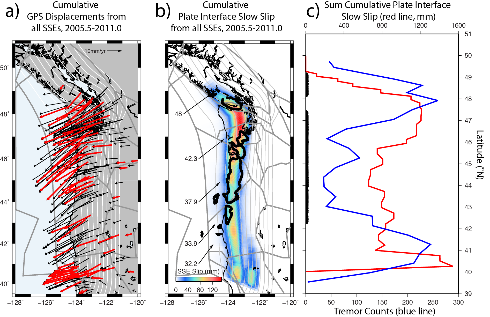
Figure 10. Figure from Schmalzle et al., 2014. (a) Sum of all SSE displacements detected at GPS (red and black vectors) from 2005.5-2011. Red vectors indicate sites that were in operation for 90% of the study. (b) Summed plate interface slow-slip from 2005.5 to 2011. Black vectors are North America relative convergence rates and directions. Thick, solid black lines mark the 10 mgal gravity anomaly contour of Blakely et al., 2005. (c) Cumulative node depth profile interface slow-slip from 2005.5 to 2011 (red line) and 50 km binned cumulative tremor counts from 2009.8 to 2013.0 acquired from the Pacific Northwest Seismic Network tremor catalog (blue line). Thick black line represents latitudes with high gravity anomalies.

Let's recap our observations:

1. Brudzinski and Allen, 2007 demonstrate using GPS and seismometers that SSEs and non-volcanic tremor detection times are segmented (Figure 5). In other words, between 40 and about 43 degrees north, ETS occurs about once every 10-11 months, ~24 months between 43 and 46-47 degrees north, and about every 14 months north of 47 degrees north.
2. Tectonic tremor counts are increased south of 43 degrees N and north of 47 degrees N (Figure 6 and Figure 10c, blue line).
3. Slow slip peaks in northern California and Washington, but is suppressed in Oregon (Figure 10).

These observations sound awfully reminiscent of the observations in my last blog post. The observations there were:

4. Reduced uplift between major subduction zone earthquakes along the coast between 43 and 46 degrees latitude (Schmalzle et al., 2014).
5. Reduced paleoseismically derived subsidence for multiple Cascadia earthquakes between 43.5 and 46 degrees latitude (Leonard et al., 2010).

In the last blog post, I talk about how observations 4 and 5 could be explained by persistent fault creep; in other words, if the fault is slipping in between large earthquakes, then it is slowly relieving stress that would have built up if the plates were stuck together. This results in less subsidence during an earthquake, and less coastal uplift between earthquakes. This idea is taken one step further and we suggest that the Siletzia terrane may be the culprit behind the persistent fault creep. The Siletzia terrane is a dense, accreted basalt that can be mapped with gravity surveys (Blakely et al., 2005). The 10 mgal gravity anomaly is plotted as a thick red line in Figure 6 and a thick black line in Figure 10b. We suggest something similar to the conceptual model presented by Reyners and Eberhart-Phillips, 2009, where the Siletzia terrane, if impermeable (i.e., water cannot pass through it), increases pore fluid pressures at the fault by not allowing water to percolate into the overriding crust. High pore fluid pressures at or near the plate interface encourages creep, since these conditions are thought to promote fault slip (Segall and Rice, 1995; Hillers and Miller, 2006).

Brudzinski and Allen, 2007 noted that the thickest accumulations of Siletzia terrane near the coast were also the regions that experience major slow slip and non-tectonic tremor events less often. In Schmalzle et al., 2014 we see that the total amount of tremor and the total amount of slow slip is also reduced in the region. But what does that mean???

Similar to the arguments posed for locking, Audet et al., 2010 suggest that fluids trapped beneath a seal at the plate boundary increase pore fluid pressures. Although the plates in the region of slow slip are stuck most of the time, they suggest that the increased pore fluid pressures allow the plates to slip with small changes in stress. They suggest that once the fault begins to slip, the pore fluid pressure decreases and the plates become stuck again, stopping the slow slip and re-enforcing the new seal. You can imagine then, that variations in the permeability of the upper crust could influence the occurrence of periodic slow slip. If the Siletzia terrane is less permeable, then it may offer a stronger seal than surrounding regions, producing higher pore fluid pressures, which may encourage more of a partial fault creep environment than one that periodically slips.

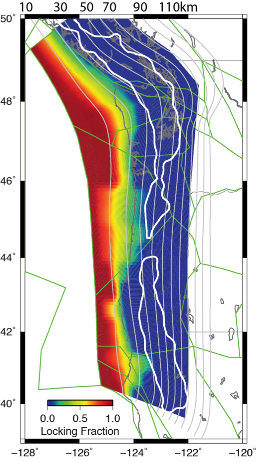
Figure 11. Map of the Cascadia subduction zone, with the Gamma-style locking model of the subduction fault presented in my previous post. Red indicates areas that are completely stuck, blue areas that are freely slipping. Colors between red and blue indicate regions that are partially creeping. White line marks the region where 95% of non-volcanic tremor occurred between 2009-2012.

Figure 11 is a map that contains the results from the Gamma-style locking model described in my previous post, where red represents areas that are estimated to be completely stuck, and blue represents areas that are freely slipping. The colors in between represent regions that are partially creeping. Also plotted is an outline of where 95% of the tremor occurred between 2009 and 2012. Together, it shows that partial fault creep is up-dip of the tremor. The conundrum here is: if persistent partial fault creep is occurring up-dip of the zone of tremor and slow slip, then wouldn't this increase the stress on the region of tremor and periodic slow slip and foster more slow slip events? If so, then why do we see the opposite -- we see less tremor and slow slip where we have more persistent fault creep! We suggest that the partial fault creep must extend into the zone of non-volcanic tremor and slow slip. Both the locking and the periodic slow slip are thought to be promoted by high pore fluid pressures. So, as fluid pressure increases due to a better seal (maybe the Siletzia?), perhaps persistent partial fault creep is the dominant mode of slip. If correct, then it is possible that the make up of the over-riding crust may determine if the fault slips as ETS or persistent fault creep (Peng and Gomberg, 2010).

For a deeper discussion of the observations and hypotheses presented in this blog, please read Schmalzle et al., 2014.

Thanks for reading and keep in touch! Contents of this blogsite are updated at http://geodesygina.com/. See other contact information below.

Acknowledgments: This work was funded by the National Science Foundation (NSF) Postdoctoral Fellowship Program, award 0847985 (Schmalzle), NSF award EAR-1062251 (McCaffrey), and USGS National Earthquake Hazards Reduction Program, Award G12AP20033 (Schmalzle and Creager). Some of the figures I made myself using General Mapping Tools (GMT), but some figures I took from random places on the web. For any of those images I say where the figure was taken. Many thanks to Reed Burgette and an anonymous reviewer for their thoughtful comments and suggestions that greatly improved this research. Thanks to Mike Brudzinski and Aaron Wech for providing their tremor catalogs. Thanks to Rick Blakeley for providing gravity data. Thanks to PBO and PANGA for providing access to GPS data products. Craig H. Faunce, Bruce Nelson, Steve Malone, Justin Sweet, David Schmidt, Aaron Wech, Tom Pratt, Brian Atwater, Sarah Minson, Lorraine Wolf, and Aimee Schmalzle provided useful comments and insight. Thanks to PBO and PANGA for providing access to GPS data products.