R helped me figure out how many shoes I can buy

One of the things I love about coding and data science is that I get to work on a lot of interesting problems. One of my good friends Craig Faunce Craig Faunce approached me over a beer with a problem. It seems he had been asked to determine how many items he could buy given a certain budget. Ok, if each and every item costs the same this is simple math, which has me puzzled. Of course it’s not that easy, since each and every item has a different cost. Ok, still not that difficult. It only becomes something that I think you would be interested in when he gets to the next part, where he says: "I'm asked to sample one population of items at a given rate, and then with my left-over money, determine at what rate I can afford to sample a second, totally different population of items with totally different costs per item."

Ok! We have an interesting little sampling project. Since Craig works for a large employer, he can't really divulge every gory detail about this issue, and obviously getting the real data isn't going to happen here. Besides, it sounded pretty boring to me, so I thought about something that I can relate to - shoes!

Figure 1 Ahh, too cute...

So I reframed the questions.

My first question is: If this year (hopefully during a big Sale) I were to blindly have an assigned shopper (or better yet, a blind assigned shopper) randomly buy a set percentage of the store, how much money would I spend? The reason we want to sample in this exercise is due to the fact that the answer depends on which shoes are purchased, since each one has a different price. So we are interested in building a distribution of potential outcomes from shoe-shopping, so we can build a range of likely outcomes from the adventure.

We will need the following libraries:

require(plyr)
require(ggplot2)

The actual data doesn't really matter for this exercise, so lets generate some with these parameters:

nshoe1 <- 1000            # Number of shoes in the store in the first year.
meanprice1 <- 100         # Mean price of shoes in the first year.
pricesd1 <- 50            # Standard deviation of the price of shoes in the first year.
R <- 0.01                                     # The sampling rate of my shopper in the first year.
it <- 200                                     # The number of iterations to build our distribution of outcomes.

I created a makedata function to create a dataframe in R consisting of nshoe rows with the associated price (called bucks) generated from a known distribution (in this case the normal, but who cares?) with a mean price of meanprice1 and a standard deviation of pricesd1:

makedata <- function (numberofshoes, dm, sdv){
  # Assign number of shoes
  df <- data.frame(shoes = seq(1:numberofshoes))
  # Assign random # of bucks for each shoe
  df$bucks <-  rnorm(n = numberofshoes, mean = dm, sd = sdv)
  return (df)
 }

The function sampleme samples from the dataframe that was created from the makedata function above:

sampleme <- function(dataframe, samplerate){
  # Generate a subsample of shoe numbers, then take the associated
  # bucks and stick them into sdf.
  sdf <- data.frame(shoes=sample(1:nrow(dataframe), size = (samplerate*nrow(dataframe))))
  sdf <- merge(sdf,dataframe,all.x=TRUE)
  return (sdf)
}

Finally, a third function storesamples enables the outcome of each random sample to be stored and appended to prior samples for later use:

storesamples<-function(iteration, df, sr){
  for (iter in 1:iteration){
    sdf <- sampleme(dataframe = df, samplerate=sr)
    sdf$index <- iter
    ifelse(iter == 1, allsdf <-sdf, allsdf <-rbind(allsdf,sdf))
  }
  return(allsdf)
}

Note that the function storesamples calls function sampleme.

Now that I have my functions, let's figure out how much money I spend if I buy 1% of the store's inventory:

# make a dataframe
shoesinstore1 <- makedata(nshoe1, meanprice1, pricesd1)
# calculate how much $$ you spent by buying 1% of the inventory
moneyIspent <- storesamples(it,shoesinstore1,R)

Now let's make a summary of the money I just spent and print it out:

summarya <- ddply(moneyIspent, .(index), summarize, Totalbucks = floor(sum(bucks)))
summary(summarya$Totalbucks)

In my last run, here are my results:

Min. 1st Qu.  Median    Mean 3rd Qu.    Max.
604.0   897.8  1009.0  1010.0  1120.0  1383.0

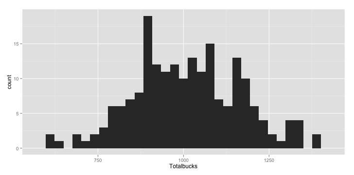
So I can expect my blind shopper to come back with a Visa/AmEX/Mastercard charge of around a thousand bucks, but it could be as low as $600, or as high as $1383 (still within my spending limit- whew!). Now let's plot our results using a histogram:

 (ggplot(summarya, aes(x=Totalbucks))
+ geom_histogram()
 )

This gives you:

Now for my second question. The following year I am given the same amount of money I spent last year as my budget. What percentage of the store's inventory in year 2 can I buy given the amount of money I spent last year?

Here we have reversed the sampling question from year 1: instead of sampling at a fixed rate to generate a distribution of credit card debts, we now have a distribution of available spending limits, and are asked to generate a distribution of expected percentage of the store purchased.

To ensure we don't go over our budget, we can't create a single sample of a given number of shoes as above- we have to select a single pair of shoes, evaluate its cost against our remaining funds, and then repeat until we have no more money. Of course in addition we need to count the number of shoes. We select each pair of shoes and conduct our evaluation with our shoesIcanbuy function:

shoesIcanbuy <- function(dataframe,mypurse){
numofshoepairs <- 0
while (mypurse > 0)  {
    Shoe.pair<-dataframe[sample(nrow(dataframe),1),] # Pick a random pair of shoes
    if (mypurse >= Shoe.pair$bucks){                 # As long as I have enough money in my purse
      mypurse<-mypurse-Shoe.pair$bucks               # Buy a pair of shoes and subtract their price from my budget
      numofshoepairs <- numofshoepairs + 1           # Record the number of shoes I bought
    }
    else {
      break
    }
  }
  return(numofshoepairs)                             # Return the number of shoes I bought
}

However the above function only gets us so far- our real interest lies in the summary of multiple shoe-shopping extravaganzas, which- you guessed it- we will conduct with another function:

how_many_shoes_in_store_I_bought <- function(dataframe, summarya, it){
  numofshoepairs <- array()                             # Declare an array
  for (i in 1:nrow(summarya)) {                         # Use each row in summarya as my starting budget
    mypurse<-summarya[i,2]
    for (j in 1:(it)){                                # Figure out how many shoes I bought with each starting budget
      numofshoepairs[j] <- shoesIcanbuy(dataframe, mypurse)
    }
    numofshoepairs.df<-data.frame(Shoes=numofshoepairs)
    ifelse(i==1, numofshoepairs.masterdf<-numofshoepairs.df,
           numofshoepairs.masterdf<-rbind(numofshoepairs.masterdf,numofshoepairs.df))
  }
  return(numofshoepairs.masterdf)
}

Now let's make this a little more realistic by making a completely different shoe line-up in the store for year 2:

shoesinstore2 <- makedata(nshoe2, meanprice2, pricesd2)

Now collect information on how many shoes I bought, and the corresponding percentage of how many shoes I bought in the store:

numofshoepairs.masterdf <- how_many_shoes_in_store_I_bought(shoesinstore2,summarya,it)

Calculate a percent of the store by taking the number of shoes I bought and dividing it by the corresponding number of shoes in the store, and multiplying by 100:

numofshoepairs.masterdf$Percent<-(numofshoepairs.masterdf$Shoes/nrow(shoesinstore2))*100

OK, let's see how much of the store I bought out:

summary(numofshoepairs.masterdf$Percent)

which gives:

   Min. 1st Qu.  Median    Mean 3rd Qu.    Max.
0.2143  0.5000  0.5714  0.5736  0.6429  1.0710

and how many shoes I bought:

summary(numofshoepairs.masterdf$Shoes)

which gives:

Min. 1st Qu.  Median    Mean 3rd Qu.    Max.
3.000   7.000   8.000   8.031   9.000  15.000

So, I bought about 8 pairs of shoes.

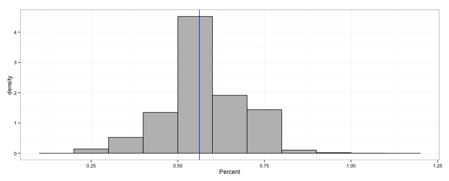
Finally, let's plot a histogram of the percentage of shoes in the store I bought:

(ggplot(numofshoepairs.masterdf, aes(x=Percent))
 + geom_histogram(aes(y=..density..), fill="gray", color="black", binwidth = .1)
 + theme_bw()
 + geom_vline(x=mean(numofshoepairs.masterdf$Percent), color="blue")
)

And you get:

And that's our shoe-shopping adventure: Sampling with the built-in function of sample in R, where we determined the size of a single sample through our rate, and secondly with the supplied function where we sample individual elements in a population and evaluate each outcome against a set threshold. Sampling forwards and backwards- have fun, and good shopping!

Interested in getting your hands on the code? Check it out in my Github Repo.