In Part 1 Creating a Database with SQLite3 we built a database. In Part 2 Populating an SQLite Database using Python we inserted values into TABLES within our database using Python 3.4 and SQLite3. Here we continue using the functionality of Python 3.4 to retrieve and visualize forecasts contained within our database. Again, I cannot thank enough David Branner, for his efforts with this project!
Our desired end-product will be to produce the map below of the differences between forecasts that were made for a specific calendar day and the forecast for that day.
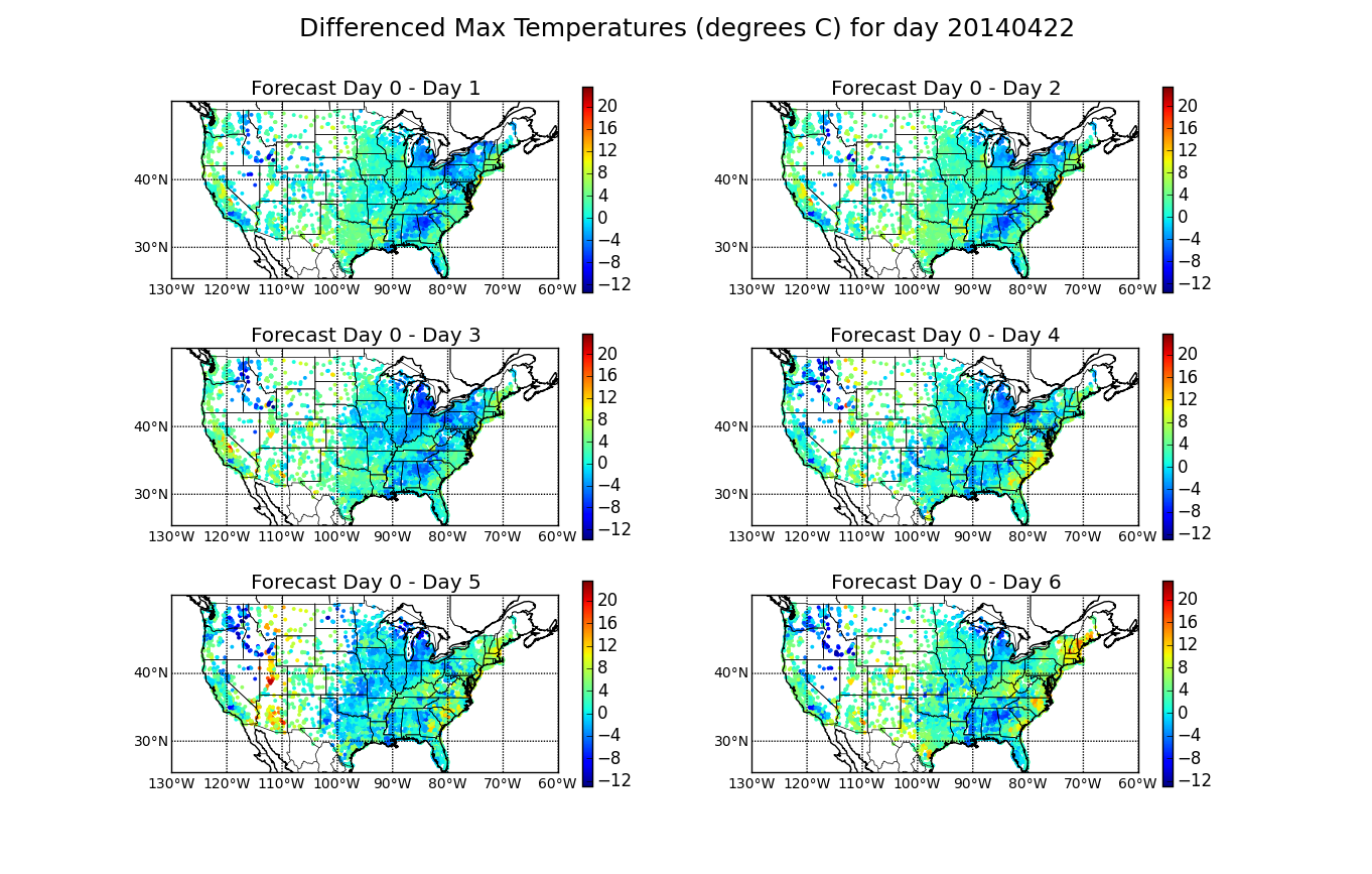
Figure 1. Maps of forecasted differences (the difference between the day of forecast and the forecast for X days out).
Part 3. Retrieving data from an SQLite Database using Python
First we need to retrieve the weather forecast data we made in the previous posts. Our database contains the forecasted maximum temperature (maxt), minimum temperature (mint), rain and snow for a given day that were made the day of to fourteen days prior. So, we need to be able to extract this information from the database. This code uses the sqlite3 module in python to extract the information:
import os
import sqlite3
def get_single_date_data_from_db(exact_date, db='weather_data_OWM.db'):
    """Retrieve forecasts for single date."""
                # exact date should be in the form YYYYMMDD
    connection = sqlite3.connect(db)
    with connection:
        cursor = connection.cursor()
        try:
            cursor_output = cursor.execute(                     # This should all be old hat to you now...
                '''SELECT lat, lon, '''
                '''maxt_0, mint_0, rain_0, snow_0, '''
                '''maxt_1, mint_1, rain_1, snow_1, '''
                '''maxt_2, mint_2, rain_2, snow_2, '''
                '''maxt_3, mint_3, rain_3, snow_3, '''
                '''maxt_4, mint_4, rain_4, snow_4, '''
                '''maxt_5, mint_5, rain_5, snow_5, '''
                '''maxt_6, mint_6, rain_6, snow_6, '''
                '''maxt_7, mint_7, rain_7, snow_7, '''
                '''maxt_8, mint_8, rain_8, snow_8, '''
                '''maxt_9, mint_9, rain_9, snow_9, '''
                '''maxt_10, mint_10, rain_10, snow_10, '''
                '''maxt_11, mint_11, rain_11, snow_11, '''
                '''maxt_12, mint_12, rain_12, snow_12, '''
                '''maxt_13, mint_13, rain_13, snow_13, '''
                '''maxt_14, mint_14, rain_14, snow_14 '''
                '''FROM locations, owm_values '''
                '''ON owm_values.location_id=locations.id '''
                '''WHERE target_date=?''', (exact_date,))
        except Exception as e:                                                                                                                  # What exceptions may we encounter here?
            print(e)
    retrieved_data = cursor_output.fetchall()                   # We receive list of simple tuples from database.
    composed_data = generate_dict_of_tuples(retrieved_data)     # Now we need to build some function that converts the retrieved data into a dictionary.
    return composed_data
Note the line:
composed_data = generate_dict_of_tuples(retrieved_data)
Here we need some way to make a usable form of the dataset. In this case the function generate_dict_of tuples receives the raw data from the SQLite3 database and converts it into a more usable dictionary of tuples:
def generate_dict_of_tuples(retrieved_data):
    """Compose the data into a succinct dictionary of tuples."""
    # Our re-composed data type is a dictionary of tuples.
    # Each tuple contains three items:
    #     sub-tuple containing latitude and longitude (floats);
    #     list of 15 sub-sub-tuples, each containing
    #         maxt, mint, rain, snow (floats).
    # For dates where the database contains no data, the forecast tuple
    # would be: `(None, None, None, None)` but this is replaced by `None`,
    # using an `if-else` clause.
    composed_data = {}
    for item in retrieved_data:
        lat_lon = item[0:2]
        forecasts = [subitem
                    if subitem[0] or subitem[1] or subitem[2] or subitem[3]
                    else None
                for subitem in
                zip(item[2::4], item[3::4], item[4::4], item[5::4])]
        composed_data[lat_lon] = forecasts
    return composed_data
Now having both of these functions in place, if we run:
get_single_date_data_from_db(20140522)
We get a dictionary that looks like this:
 {(38.576698, -92.173523): [(18.71, 6.97, 0, 0),
 (21.03, 8.7, 0, 0),
 (20.67, 9.72, 0, 0),
 (19.01, 7.23, 0, 0),
 (22.08, 9.07, 0, 0),
 (21.68, 9.53, 0.34, 0),
 (22.33, 10.22, 0, 0),
 (16.18, 12.14, 1.23, 0),
 (19.05, 12.02, 10.08, 0),
 None,
 None,
 None,
 None,
 None,
 None],
(34.154179, -117.344208): [(17.37, 6.16, 0, 0),
 (19.66, 7.48, 0, 0),
 (21.24, 6.27, 0, 0),
 (21.71, 5.5, 0, 0),
 (18.34, 8.88, 0, 0),
 (20.78, 4.73, 0, 0),
 (20.78, 4.73, 0, 0),
 (22.96, 7.06, 0, 0),
 (20.78, 4.73, 0, 0),
 None,
 None,
 None,
 None,
 None,
 None],
       .
       .
       .}
The keys are the location's latitude and longitude, and the values are the forecasts. In this example we have 9 forecasts: one for the day of and 8 days out (other values that are not present are marked as ‘None’).
Fabulous. In Figure 1 we focus only on the maximum temperature (maxt) forecasts. We visualize the absolute differences between the maximum forecasted values for the day of and the forecasted value for that day at some time in the past. The differenced values are presented on a map of the United States using warm colors to reflect that the forecast the day of was warmer and cooler colors to reflect cooler temperatures (pun intended). With our data extracted, we need only to calculate the differences and we will plot the data using python's matplotlib with the basemap toolkit.
This visualization will include six subplots- one for each successive day leading up to our target date. Thinking about this another way, if our target date is April 22, 2014 (20140422), and we assign that the letter t, then we are making a subplot for differences between t, the day of forecast, and the forecast made at t-1, t-2, t-…n days.
To collect the data for our target date we run the function below, which makes lists containing the latitude, longitude and differences, and sends them off to be processed by our next function:
def make_map(target_date=20140422):
'''Make a basic map of the United States'''
# target_date is the day the forecasts were made for
lat=[]; lon=[]; diff=[]
forecasts = get_single_date_data_from_db(target_date)                           # Call earlier function to get dictionary
for city in forecasts:
        # First collect the lats and longs of the cities
        lat.append(city[0])
        lon.append(city[1])
        #Collect differenced maxt values
        diff.append([
                (forecasts[city][0][0]-forecasts[city][1][0]),
                (forecasts[city][0][0]-forecasts[city][2][0]),
                (forecasts[city][0][0]-forecasts[city][3][0]),
                (forecasts[city][0][0]-forecasts[city][4][0]),
                (forecasts[city][0][0]-forecasts[city][5][0]),
                (forecasts[city][0][0]-forecasts[city][6][0]),
                (forecasts[city][0][0]-forecasts[city][7][0]),
                (forecasts[city][0][0]-forecasts[city][8][0])])
make_basemap(lon,lat,diff,target_date)                                                                                  # Send this information to make_basemap --> our next function!
plt.show()
The second function we have named "make_basemap”, and does the mapping work:
import numpy as np
import matplotlib.pyplot as plt
from mpl_toolkits.basemap import Basemap, cm
def make_basemap(lon,lat,diff,target_date):
        for day in range(1,7):                                                                                                                                          # Run this for each forecasted difference
                subdiff = []
                for city in range(0,len(diff)):
                        subdiff.append(diff[city][day])
                plt.subplot(3,2,day)                                                                                                                                            # Define where the subplot will lie on figure
                mindiff = min(subdiff)
                maxdiff = max(subdiff)

                # create Mercator Projection Basemap instance.
                m = Basemap(projection='merc',\
                                                                llcrnrlat=25,urcrnrlat=50,\
                                                                llcrnrlon=-130,urcrnrlon=-60,\
                                                                rsphere=6371200.,resolution='l',area_thresh=10000)
                # draw coastlines, state and country boundaries, edge of map.
                m.drawcoastlines()
                m.drawstates()
                m.drawcountries()
                # draw parallels.
                parallels = np.arange(0.,90,10.)
                m.drawparallels(parallels,labels=[1,0,0,0],fontsize=10)
                # draw meridians
                meridians = np.arange(180.,360.,10.)
                m.drawmeridians(meridians,labels=[0,0,0,1],fontsize=10)

                # draw Circles on the map
                # Determine min and max differenced values
                jet = plt.cm.get_cmap('jet')
                x,y = (m(lon,lat))
                sc = plt.scatter(x, y, c=subdiff, vmin=mindiff, vmax=maxdiff, cmap=jet, s=8, edgecolors='none' )
                # add colorbar
                plt.colorbar(sc)
                # add title
                plt.suptitle("Differenced Max Temperatures (degrees C) for day "+str(target_date), fontsize=18)
                plt.title("Forecast Day 0 - Day "+str(day))
Executing make_map() we get the Figure 1. Note that a subplot is created for each differenced forecast through a for loop which also defines the subplot being created.
Like what you see? Stay tuned, the next step on my agenda is making an interactive website that will allow users to play with the data! Thanks for reading!
Comments
comments powered by Disqusblogroll
social