Elastic Half Space Model of a Vertical Strike Slip Fault

In between major earthquakes, the ground deforms due to movement of tectonic plates. For strike-slip faults, such as the San Andreas Fault, the ground deforms in an 'S' shape that can be modeled as an arctangent. To better understand what is observed at the surface, imagine a fence built perpendicularly across a strike-slip fault. When the fault is first built it is nice and straight, but over time it starts to deform and look kind of like an "S". When the earthquake occurs the ground (and the fence) will snap, and the two sides of the fence will become straight again at some time after the earthquake, although displaced.

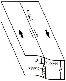
Figure 1. Deformation of tectonic plates between major earthquakes. D is the locking depth (the depth at which the fault is stuck). Figure modified from http://geologycafe.com/california/pp1515/chapter7.html

A simple model of this movement for vertical strike slip faults in a homogenous elastic half space [Weertman and Weertman, 1964; Savage and Burford, 1973] can be described as:

V(x) = (vo/pi)arctan(x/D)

where V(x) is the velocity of points estimated along a perpendicular profile across the fault, v is the far field velocity, x is the distance from the fault, and D is the dislocation depth.

High precision GPS can be used to observe the deformation around fault systems. The velocity, position and uncertainty estimates can be compared directly to the model to estimate the goodness of fit of the model. The chi2 statistic is give by:

chi2 = SUM ((dataR -vel)/(sig))**2

where chi2 = chi2 statistic, dataR = GPS estimated rate for a position aling the profile, vel = model calculated velocity, and sig = GPS velocity uncertainty. SUM is the sum of all chi2 for each GPS datum.

The reduced chi2 is also calculated and is given by:

reduced chi2 = chi2 / (N-v-1)

where N = number of data, v = number of variable parameters (in this case 2, R and d). An ideal reduced chi2 should equal 1.

In this blog, I use high precision GPS velocities from Schmalzle et al, [2006], and compare them to the model described above. I use the chi2 statistic and the reduced chi2 to determine the goodness of fit of the model to the data. My githup repo has versions of how to do this in Fortran with visualization using General Mapping Tools (GMT), and how to do it in Python. This blog will cover only the techniques used in the Python version of the code.

I have a few external files that are read in the code and are also available in the my githup repo. The file param.py holds the values of the far field velocity and locking depth for a given model run and looks like this:

xmin=-150.
xmax=150.
int=1.
Vo=34.
d=15.
dmin=1.
dmax=100.
Vmin=0.
Vmax=100.

The file data.py contains the GPS data in the form of x (in km), Rate (in mm/yr) and uncertainty (in mm/yr) and looks like this:

-92.60814 15.0918 -3.561012106
-90.65163 15.4416 -3.592941176
-92.60814 15.1681 -1.42072184
-71.08653 14.3386 -1.661513002
-69.13002 16.4146 -1.773867193
-47.60841 10.1976 -1.511861585
-60.65181 14.0536 -1.95124564
-70.43436 14.4541 -2.901815856
-2.282595 0.82942 -1.622786425
-27.39114 8.70825 -1.672086072
0.65217 0.18103 -1.550890689
7.499955 -6.89121 -1.799743676
19.5651 -11.9668 -1.632284566
-17.60859 4.82287 -1.62481939
12.39123 -8.5554 -1.223772558
33.91284 -15.2699 -1.190422007
65.86917 -15.6106 -1.351439143
122.60796 -15.6614 -6.776253439
3.26085 -5.95536 -1.524006894
2.60868 -2.39876 -1.179208687
6.5217 -5.81965 -1.62421975
-13.0434 5.08107 -1.23548631

Now for the coding! First, import the following modules:

import numpy as np
import math
import matplotlib.pyplot as plt

and import the param.py file:

import param

I collect the information from the param file and computed the surface velocities like this:

f = open('vel.txt','w')
listx = []
listVel = []
x=param.xmin
while (x <= param.xmax):
    Vel=-((param.Vo/np.pi)*math.atan(x/param.d))
    print >> f, x, Vel
    listx.append(x)
    listVel.append(Vel)
    x = x + param.int

This calculates the predicted velocity for a defined increment along a profile of a strike slip fault. I keep the x's and calculated velocities in lists that will be used later in the program for plotting purposes.

Now let's open the GPS file and read its contents:

g=np.loadtxt('data.py')
gx = g[:,0]
gVel = g[:,1]
gsig = g[:,2]

Now calculate the expected velocity or at each GPS position:

VelC = -((param.Vo / np.pi) * np.arctan ([ gx/param.d ]))

and calculate the chi2 and reduced chi2

chi = ((gVel - VelC)/ (gsig))**2
chi2 = sum(chi.T)
redchi = chi2/(len(gVel)-3)

Now you have the model fit to the data for a modeled fault rate and locking depth! The model fit to the data looks like Figure 2.

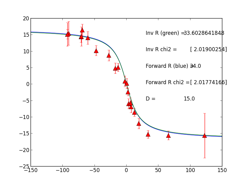
Figure 2. Modeled velocities across a vertical strike slip fault (solid lines) compared to GPS velocities (triangles) with velocity uncertainty error bars. Both gridsearch estimated and inversion estimated low misfit rates are shown for a locking depth of 15km. The reduced chi2 is given.

But suppose you want to know which combination of modeled fault rate and locking depth give you the best fit to the data. One way you can do this is by running a whole suite of models that include different combinations of fault rate and locking depth values. This is called a gridsearch approach, and is perhaps the simplest (although most time consuming) method. The param.py files contains user input values for a range of modeled parameters. Grabbing those values we can then perform a while loop to loop through those ranges:

dmin=param.dmin
dmax=param.dmax
Vmin=param.Vmin
Vmax=param.Vmax

d=param.dmin
gridredchi = np.array([V, d, chi])
grc = []
c = open('chi.py','w')

while (d <= dmax):
 V=param.Vmin
 while (V <=  Vmax):
   gridVelC = -((V / np.pi) * np.arctan ([ gx/d ]))
   gridchi = ((gVel - gridVelC)/ (gsig))**2
   gridchisum = np.matrix.item(sum(gridchi.T))
   gridrchi= gridchisum/(len(gVel)-3)
   newrow =  [ V, d, gridrchi ]
   gridredchi = np.vstack([gridredchi, newrow])
   print >> c, V, d, gridrchi
   plt.scatter(V,d, c=gridrchi, marker='s',lw=0,  s=40, vmin=0, vmax=10)
   V = V + param.int
 d = d + param.int

By performing the gridsearch, you can contour the estimated chi2 value with the defined model rate and locking depth as shown in Figure 3.

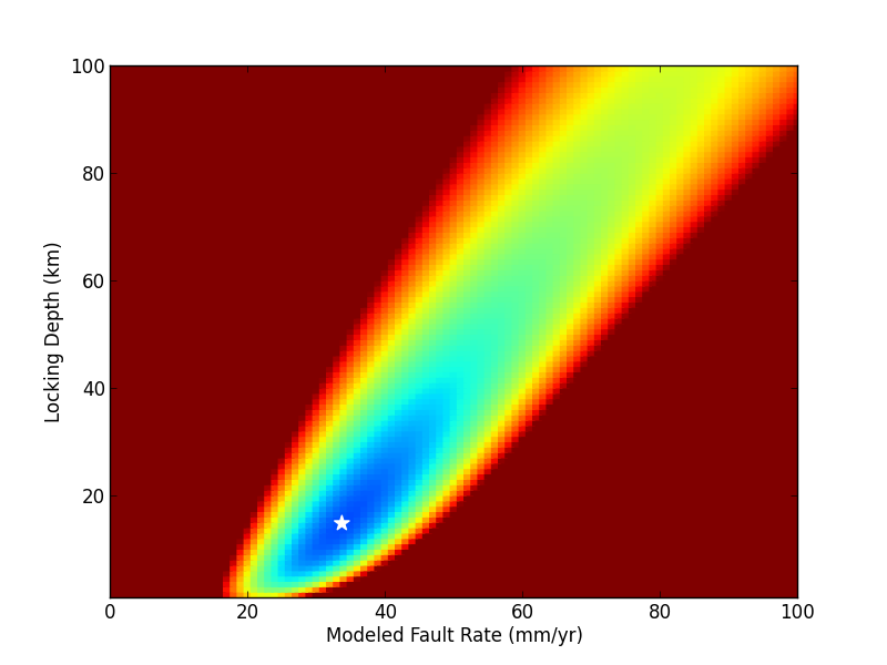
Figure 3. Contour plot of the chi2 statistic (colors, cooler colors indicate lower misfit) given modeled values of fault rate and locking depth. The white star marks the low misfit model.

Performing a gridsearch can take a long time, but it has the advantage that it is a straightforward method to estimate the low misfit model. By imaging our chi2 distribution, like in Figure 3 we can also easily see if there are other minima that could provide an alternative model that fits the data just as well for our given parameter ranges. The down side, however, is that this method is really slow, especially for more complicated models that require longer computation times.

An alternative method is to linearly invert the data with a little bit of matrix algebra. A great book that clearly describes this technique is:

Aster, R., Borchers, B., Thurber, C., Parameter Estimation and Inverse Problems, 301 pp, Elsevier Academic Press, 2004.

I highly recommend this book for further reading on this subject. I am not going to go over these concepts in this blog, but these methods are used in the scripts in my github repo. I use a linear inverse approach which is only valid for linear parameters, hence I can use it to estimate the best fitting rate, but not the locking depth. Using this method, the model is run for a locking depth of 15 km to find the best fit model in Figure 2.