Global Positioning Systems

Global Positioning Systems (GPS) are used to measure the three dimensional position of a point over time. High precision GPS are used to measure tectonic plate motion by measuring the position of a permanently installed geodetic monument over time. The GPS instruments are either permanently installed over the monument and continuously recording its position over time, or the GPS monuments are perodically measured. With either method, three dimensional position estimates are made over time.

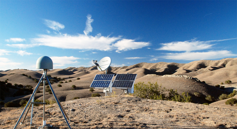
This is an image of a high precision GPS antenna, whose image I took from the UNAVCO website:

And this is an example of the GPS site BEMT position 3D time series taken from UNAVCO:

Blue dots are daily position estimates in the north (top), east (middle) and vertical (bottom) components. This site experienced an offset due to an earthquake in 2010. For more information on how GPS works, please visit: http://www.unavco.org/edu_outreach/teachers/teachers.html

GPS Velocities

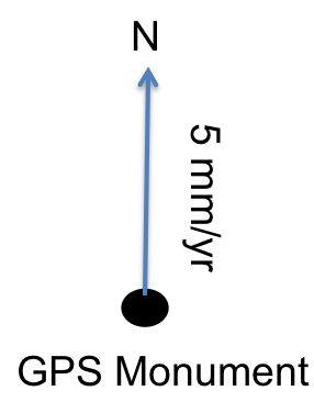
The rate at which a geodetic monument moves can be estimated by taking the slope of the time series for each component. Take for example the time series shown above. This is going to be a rough estimate, but between 2004 and 2010, the monument north component position moved from -15 mm to +15 mm, totalling 30 mm of displacement over 6 yrs, indicating that it is moving at 5 mm/yr in the north position.

Using the same logic, the east component moved ~-50 mm over about 6 years, giving the east component a rate of 8.3 mm/yr to the west.

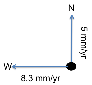
The Magnitude and direction of the horizontal GPS velocity vector can now be calculated:

Vector Projection

In map view small variations in GPS velocities may be difficult to see, hence it is sometimes useful to plot GPS velocities along a profile. The profile line can follow a fault line, and, if it does, one can calculate the fault parallel and perpendicular components of motion. Fault parallel motion will give you an idea of lateral motion across the fault (as in strike-slip fault systems), and fault perpendicular motion will tell you if the two sides of the fault are separating or converging. In this section, we will talk about deriving the profile parallel and perpendicular components of the GPS vectors using vector projection.

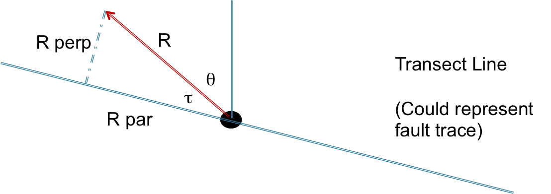
Here the fault perpendicular velocity is: R perp= R*sin(t) and the fault parallel velocity is: R par= R*cos(t)

The Vector Projector

Stuart Sandine, Andrea Fey and Thomas Ballinger and I created a web app called The Vector Projector that calculates the magnitude, transect parallel and transect perpendicular components of GPS velocities along a profile. In this app, you are given the option of several GPS velocity fields, calculated with respect to stable North America. For now you can choose your profile width and you can filter what data you would like to use by their uncertainties (i.e., uncertainties that are more than the value specified are not used). This beta version does not plot uncertainties, which we plan to change in the future. Give it a try! Go to the Vector Projector.